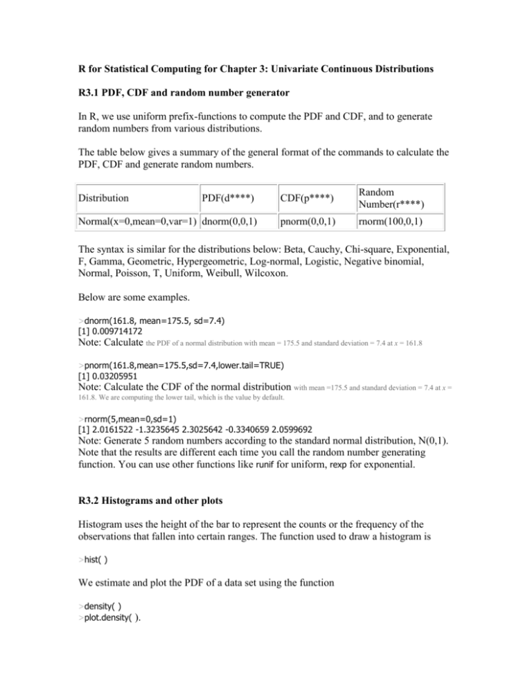
R for Statistical Computing for Chapter 3: Univariate Continuous Distributions
R3.1 PDF, CDF and random number generator
In R, we use uniform prefix-functions to compute the PDF and CDF, and to generate
random numbers from various distributions.
The table below gives a summary of the general format of the commands to calculate the
PDF, CDF and generate random numbers.
PDF(d****)
CDF(p****)
Random
Number(r****)
Normal(x=0,mean=0,var=1) dnorm(0,0,1)
pnorm(0,0,1)
rnorm(100,0,1)
Distribution
The syntax is similar for the distributions below: Beta, Cauchy, Chi-square, Exponential,
F, Gamma, Geometric, Hypergeometric, Log-normal, Logistic, Negative binomial,
Normal, Poisson, T, Uniform, Weibull, Wilcoxon.
Below are some examples.
>dnorm(161.8, mean=175.5, sd=7.4)
[1] 0.009714172
Note: Calculate the PDF of a normal distribution with mean = 175.5 and standard deviation = 7.4 at x = 161.8
>pnorm(161.8,mean=175.5,sd=7.4,lower.tail=TRUE)
[1] 0.03205951
Note: Calculate the CDF of the normal distribution with mean =175.5 and standard deviation = 7.4 at x =
161.8. We are computing the lower tail, which is the value by default.
>rnorm(5,mean=0,sd=1)
[1] 2.0161522 -1.3235645 2.3025642 -0.3340659 2.0599692
Note: Generate 5 random numbers according to the standard normal distribution, N(0,1).
Note that the results are different each time you call the random number generating
function. You can use other functions like runif for uniform, rexp for exponential.
R3.2 Histograms and other plots
Histogram uses the height of the bar to represent the counts or the frequency of the
observations that fallen into certain ranges. The function used to draw a histogram is
>hist( )
We estimate and plot the PDF of a data set using the function
>density( )
>plot.density(
).
To calculate the CDF of a data set, use the function
>ecdf( )
To generate Figure 3.1, we use (substitute k = 10, 100, 1000):
>hist(runif(1000000), breaks=k, prob=T, main="Histogram for Uniform (0,1)",xlab=" X Values
",ylab="Probability").
To generate Figure 3.2, we use
>plot(cbind(seq(1.401,2.1,0.001),c(rep(0,100),rep(2,500),rep(0,100))),main="PDF of U(1.5,2)",
xlab="Exchange rate (X)", ylab="PDF f(x)", ylim=c(0,2.1),type="o",lty=2);
>plot(cbind(seq(1.401,2.1,0.001),c(rep(0,100),seq(0.002,1,0.002),rep(1,100))),main="CDF of
U(1.5,2)", xlab="Exchange rate (X)", ylab="CDF F(x)", ylim=c(0,1.0),type="p",lty=1)
To generate Figure 3.3, we use
>plot(density(rnorm(1000000,mean=161.8,sd=6.9), kernel="g"),main="PDF of Normal
(161.8,6.9^2) ",xlab="Female height in cms", ylab="PDF f(x)")
>plot(ecdf(rnorm(1000000,mean=161.8,sd=6.9)),main="CDF of Normal (161.8,6.9^2)
",xlab="Female height in cms",ylab="CDF F(x)")
To generate Figure 3.4, we use
>plot(cbind(seq(0.001,200.0,0.001),0.05*exp((-0.05)*seq(0.001,200.0,0.001))),main="PDF of
Exponential (Lambda=0.05)", xlab="Waiting Time (t)", ylab="PDF f(t)", type="l",lty=1)
>plot(cbind(seq(0.001,200.0,0.001),rep(1,length(seq(0.001,200.0,0.001)))-exp((0.05)*seq(0.001,200.0,0.001))),main="CDF of Exponential (Lambda=0.05)", xlab="Waiting Time
(t)", ylab="CDF F(t)", type="l",lty=1)
To generate Figure 3.5, we use (for n=10, p=0.6)
>plot(seq(-0.5,9.5,0.001),dbinom(floor(seq(0,10,0.001)),size=10,prob=0.6)dbinom(seq(0,10,0.001),size=10,prob=0.6),main="Binomial distribution with Normal
Approximation", xlim=c(0,10), ylim=c(0,0.25),xlab="No. of Sucesses",
ylab="Probability",type="l")
>lines(density(rnorm(1000000,mean=6,sd=1.549193),kernel="g"),lty=2)