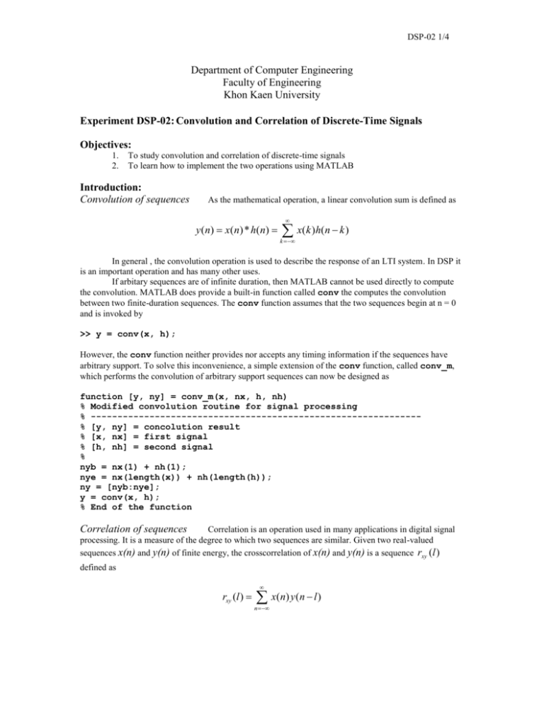
DSP-02 1/4
Department of Computer Engineering
Faculty of Engineering
Khon Kaen University
Experiment DSP-02: Convolution and Correlation of Discrete-Time Signals
Objectives:
1.
2.
To study convolution and correlation of discrete-time signals
To learn how to implement the two operations using MATLAB
Introduction:
Convolution of sequences
As the mathematical operation, a linear convolution sum is defined as
y ( n)  x ( n) * h( n) 

 x ( k ) h( n  k )
k 
In general , the convolution operation is used to describe the response of an LTI system. In DSP it
is an important operation and has many other uses.
If arbitary sequences are of infinite duration, then MATLAB cannot be used directly to compute
the convolution. MATLAB does provide a built-in function called conv the computes the convolution
between two finite-duration sequences. The conv function assumes that the two sequences begin at n = 0
and is invoked by
>> y = conv(x, h);
However, the conv function neither provides nor accepts any timing information if the sequences have
arbitrary support. To solve this inconvenience, a simple extension of the conv function, called conv_m,
which performs the convolution of arbitrary support sequences can now be designed as
function [y, ny] = conv_m(x, nx, h, nh)
% Modified convolution routine for signal processing
% -------------------------------------------------------------% [y, ny] = concolution result
% [x, nx] = first signal
% [h, nh] = second signal
%
nyb = nx(1) + nh(1);
nye = nx(length(x)) + nh(length(h));
ny = [nyb:nye];
y = conv(x, h);
% End of the function
Correlation of sequences
Correlation is an operation used in many applications in digital signal
processing. It is a measure of the degree to which two sequences are similar. Given two real-valued
sequences x(n) and y(n) of finite energy, the crosscorrelation of x(n) and y(n) is a sequence rxy (l )
defined as
rxy (l ) 

 x ( n) y ( n  l )
n 
DSP-02 2/4
The index l is called the shift or lag parameter. The special case when y (n)  x(n) is called
autocorrelation and is defined by
rxx (l ) 

 x ( n) x ( n  l )
n 
If we compare the convolution operation with the crosscorrelation of two sequences, we observe a close
resemblance. The crosscorrelation rxy (l ) can be put in the form
rxy (l )  x(l )  y (l )
with the autocorrelation
rxx (l ) in the form
rxx (l )  x(l )  x(l )
Therefore these correlations can be computed using the conv function if sequences are of finite duration.
The signal-processing toolbox MATLAB provides a function called xcorr for sequence
correlation computations. However, the function does not provide the timing (or lag) information, which
then must be obtained by some other means.
Experiment:
( Before starting the lab, you’re supposed to have all functions from DSP-01 stored in your working folder.)
A. Convolution of Sequences
Given the following two sequences
x1(n) = [ 0, 0, 1, 1, 1, 1, 1] and

1.
2.
For –10  k  10, plot x1(k) and x2(k) using the stem function.
Plot x1(k) and x2(-k) and then with a loop control structure, write a program to determine
10
y(0) =

k 10
3.
x2(n) =[0, 0, 0, 1, 1, 1]

x1 (k ) x2 ( k )
Plot x1(k) and x2(1-k) and then, with a loop control structure, write a program to determine
10
y(1) =
 x (k ) x (1  k )
k 10
4.
1
2
Plot x1(k) and x2(-1-k) and then with a loop control structure, write a program to determine
10
y(-1) =
 x (k ) x (1  k )
k 10
5.
1
2
Develop a program to determine
y (n)  x1 (n) * x2 (n) 

 x (k ) x (n  k )
k 
1
2
15  n  15
DSP-02 3/4
6.
7.
8.
For –15  n  15, plot the sequence y(n) obtained in (5). What are the beginning point and end point of
y(n) that are non-zero values?
Invoke the following MATLAB commands and plot the result (y versus ny)
>> x1 = [0, 0, 1, 1, 1, 1, 1]; nx1 = [-3:3];
>> x2 = [0, 0, 0, 1, 1, 1]; nx2 = [-3:2];
>> [y, ny] = conv_m(x1, nx1, x2, nx2);
Compare the plot in (7) to the plot in (6). Briefly explain what you get.
B. Correlation of Sequences
1.
2.
Create a MATLAB function called xcorr_m to perform the correlation operation based on the
convolution operation.
Let x(n) = [3, 11, 7, 0, -1, 4, 2] be a prototype sequence and y(n) = x(n-2)+w(n) be its noise-corrupted

and shifted version. Write the following code and save as a M-file.
% noise sequence 1
x =[3, 11, 7, 0, -1, 4, 2]; nx = [-3:3];
% given siganl x(n)
[y, ny] = sigshift(x, nx, 2);
% obtain x(n-2)
w = randn(1, length(y)); nw= ny;
% generate w(n)
[y, ny] = sigadd(y, ny, w, nw);
% obtain y(n) = x(n-2) + w(n)
[rxy, nrxy] = xcorr_m(x, nx, y, ny);
% crosscorrelation
subplot(2, 1, 1); stem(nrxy, rxy);
axis([-5, 10, -50, 250]); xlabel(‘lag variable l’);
ylabel(‘rxy’); title(‘Crosscorrelation: noise sequence 1’);
%
% noise sequence 2
x =[3, 11, 7, 0, -1, 4, 2]; nx = [-3:3];
% given siganl x(n)
[y, ny] = sigshift(x, nx, 2);
% obtain x(n-2)
w = randn(1, length(y)); nw = ny;
% generate w(n)
[y, ny] = sigadd(y, ny, w, nw);
% obtain y(n) = x(n-2) + w(n)
[rxy, nrxy] = xcorr_m(x, nx, y, ny);
% crosscorrelation
subplot(2, 1, 2); stem(nrxy, rxy);
axis([-5, 10, -50, 250]); xlabel(‘lag variable l’);
ylabel(‘rxy’); title(‘Crosscorrelation: noise sequence 2’);
3.
Run the script saved in (2) and print the output figure.
Questions:
1.
Determine if the result sequences from A.6 and A.7 are identical or not. Explain.
2.
Let
3.
the beginning and end point of y (n)  x(n)  h(n) .
From the result in B.3, what is the value of l that the crosscorrelation got peak? What would it imply?
x(n); nxb  n  nxe  and h(n); nhb  n  nhe  be two finite-duration sequences. Determine
Nawapak Eua-anant and Rujchai Ung-arunyawee
15 November 2548
DSP-02 4/4
Name:______________________________________________________________ID:________________
In class assignment
1. Explain, step by step, the method to perform the convolution between 2 signals that you use
in part A of this experiment.
2. What knowledge do you get from this lab?