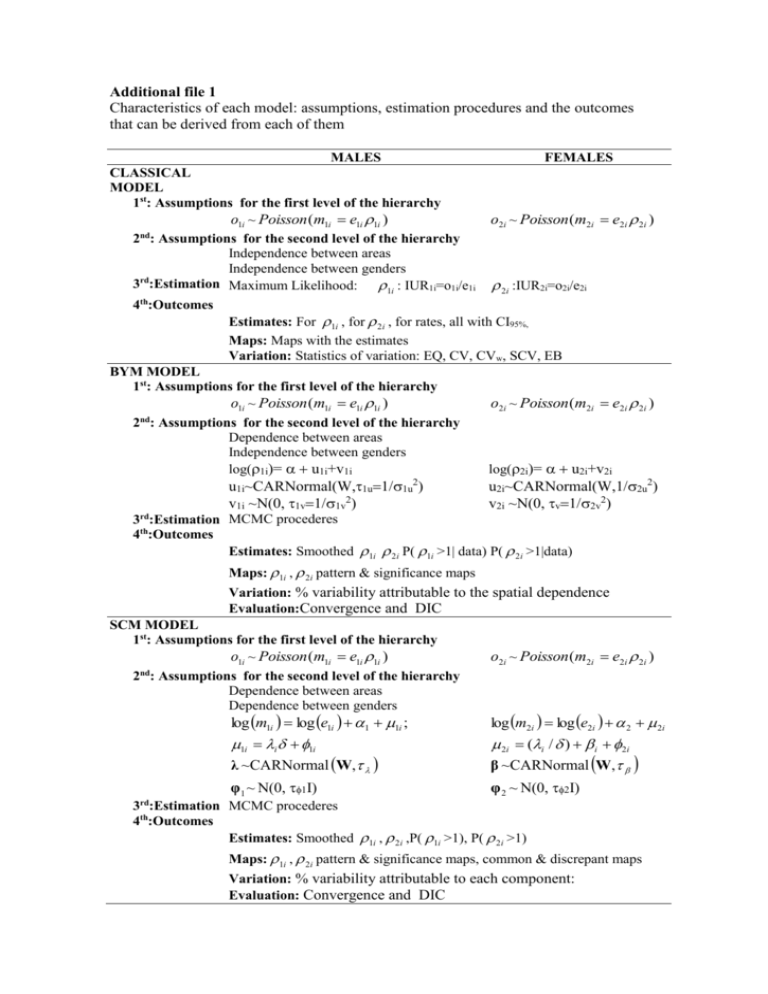
Additional file 1
Characteristics of each model: assumptions, estimation procedures and the outcomes
that can be derived from each of them
MALES
FEMALES
CLASSICAL
MODEL
1st: Assumptions for the first level of the hierarchy
o1i ~ Poisson (m1i  e1i 1i )
o2i ~ Poisson (m2i  e2i  2i )
nd
2 : Assumptions for the second level of the hierarchy
Independence between areas
Independence between genders
3rd:Estimation Maximum Likelihood:  1i : IUR1i=o1i/e1i  2i :IUR2i=o2i/e2i
4th:Outcomes
Estimates: For  1i , for  2i , for rates, all with CI95%,
Maps: Maps with the estimates
Variation: Statistics of variation: EQ, CV, CVw, SCV, EB
BYM MODEL
1st: Assumptions for the first level of the hierarchy
o1i ~ Poisson (m1i  e1i 1i )
o2i ~ Poisson (m2i  e2i  2i )
nd
2 : Assumptions for the second level of the hierarchy
Dependence between areas
Independence between genders
log(1i)= u1i+v1i
log(2i)= u2i+v2i
u1i~CARNormal(W,1u1u2)
v1i ~N(0, 1v1v2)
u2i~CARNormal(W,2u2)
v2i ~N(0, v2v2)
3rd:Estimation MCMC procederes
4th:Outcomes
Estimates: Smoothed  1i  2i P(  1i >1| data) P(  2i >1|data)
Maps:  1i ,  2i pattern & significance maps
Variation: % variability attributable to the spatial dependence
Evaluation:Convergence and DIC
SCM MODEL
1st: Assumptions for the first level of the hierarchy
o1i ~ Poisson (m1i  e1i 1i )
nd
2 : Assumptions for the second level of the hierarchy
Dependence between areas
Dependence between genders
o2i ~ Poisson (m2i  e2i  2i )
log m1i   log e1i   1  1i ;
log m2i   log e2i    2   2i
1i  i   1i
λ ~CARNormal W,   
 2i  (i /  )   i  2i
β ~CARNormal W,   
φ1 ~N(0, 
φ 2 ~N(0, 
rd
3 :Estimation MCMC procederes
4th:Outcomes
Estimates: Smoothed  1i ,  2i ,P(  1i >1), P(  2i >1)
Maps:  1i ,  2i pattern & significance maps, common & discrepant maps
Variation: % variability attributable to each component:
Evaluation: Convergence and DIC
* Notation used in previous table
Specification
Common notation
o1i , o2i
e1i , e2i
 1i ,  2i
Classic model
IUR1i, IUR2i
EQ, CV, CVw, SCV, EB
BYM model
u1i, u2i
v1i,, v2i
% variance spatially
structured
P(  1i >1| data)
P(  2i >1| data)
DIC
Explanation
Number of admissions in area i in males and in females
Number of expected admissions in area i in males and in females,
assuming common rates along the whole region
Risk of admissions in males and females in area i, unknown, needs to be
estimated
Indirect Utilization ratios, which are the estimates for  1i ,  2i via
Maximum-Likelihood IUR1i=o1i/e1i
Statistics of Variation EQ: Extremal Quotient; CV: Coefficient of
Variation; CVw: Weighted Coefficient of Variation; SCV: Systematic
Component of Variation; EB: Empirical Bayes statistic. Higher values
indicate higher variability.
Random effects which model the spatial correlation in the risk of
admission for males (u1i) and females (u2i). To do so, a conditional
autorregresive distribution is assigned for each one,
CARNormal(W,1u1u2). If data are not correlated, the variance
component estimate, 1u, will be low
Random effects which have independent structure, N(0, 1v1v2). They
need to be included together with the ui random vector, otherwise we
would be forcing spatial structure where it may not be present.
=sum2/ (sum2 + v2), where sum2 is the marginal spatial variance, sum2=∑i(ui ū)2/(n-1),
The posterior probability for area i to have an admission risk higher than
that for the whole region, given the data. These values are often used to
derive probability maps, for which cut-off points 0.2 and 0.8 are used.
Deviance Information Criteria: it is used in the Bayesian framework to
compare models. DIC=D+ pD, where D is the Deviance average and pD the
number of effective parameters. Models with smaller DIC are preferred.
SCM model
1i ,  2i
i

 i , 1i , 2i
In the log-scale, the relative risk of admission in area i for males and
females compared to that of the whole region
The random effect assigned to area i, which represents the shared risk in
males and females. We assumed it as spatially correlated.
A parameter that allows for a different gradient on the shared component
for males and females.
The random effects assigned to area i, which depict differences between
males and females with respect to the common pattern. 1i is referred to
males and  i and  2i are referred to females,  i with spatial structure
and 1i and  2i with an independent structure.
Partition of variance
P(  1i >1| data), DIC
The whole variability observed in males can be decomposed by that
attributed to the common pattern and that specific to males. The same
applies to females.
Idem explanation as for BYM model