Supplementary Information for “An analytic model for accurate spring constant calibration of rectangular atomic force microscope cantilevers”
Rui Li 1,2 , Hongfei Ye 1 , Weisheng Zhang 1 , Guojun Ma 1 & Yewang Su 3,4
In this file, we elaborate on the solution of governing equation for static problem of a rectangular AFM cantilever, by which we find the analytic scaling law [equation (5) of the main text] for spring constant calibration.
S.1. Governing equation within the framework of Hamiltonian system
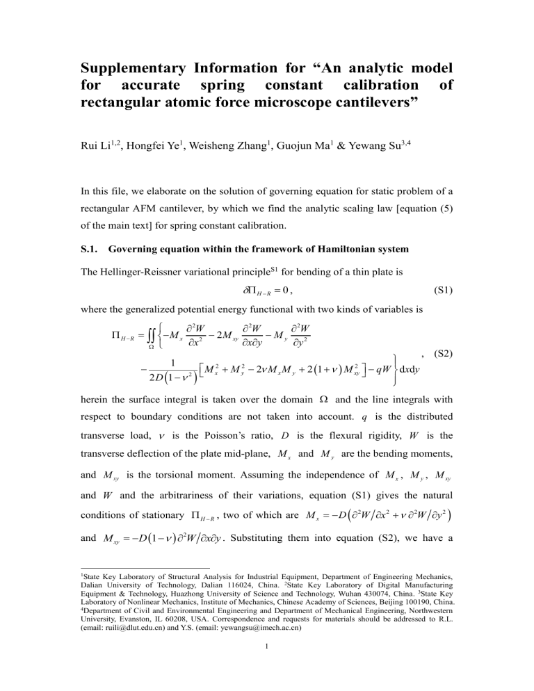
The Hellinger-Reissner variational principle
S1
for bending of a thin plate is
  
0 , (S1) where the generalized potential energy functional with two kinds of variables is
  



M x
 2
W
 x
2

2 M xy
 2
W

M y
 2
W
 y
2

2 D

1
1
 
2
 M 2 x

M 2 y

2

M M x y
    
M 2 xy

 qW d d

, (S2) herein the surface integral is taken over the domain

and the line integrals with respect to boundary conditions are not taken into account. q is the distributed transverse load,

is the Poisson’s ratio, D is the flexural rigidity, W is the transverse deflection of the plate mid-plane, M x
and M y
are the bending moments, and M xy
is the torsional moment. Assuming the independence of M x
, M y
, M xy and W and the arbitrariness of their variations, equation (S1) gives the natural conditions of stationary

, two of which are M x
 
D

 2
W x

2
W
 y
2
 and M xy
 
D

1
 
2
W x y . Substituting them into equation (S2), we have a
1 State Key Laboratory of Structural Analysis for Industrial Equipment, Department of Engineering Mechanics,
Dalian University of Technology, Dalian 116024, China. 2 State Key Laboratory of Digital Manufacturing
Equipment & Technology, Huazhong University of Science and Technology, Wuhan 430074, China. 3 State Key
Laboratory of Nonlinear Mechanics, Institute of Mechanics, Chinese Academy of Sciences, Beijing 100190, China.
4 Department of Civil and Environmental Engineering and Department of Mechanical Engineering, Northwestern
University, Evanston, IL 60208, USA. Correspondence and requests for materials should be addressed to R.L.
(email: ruili@dlut.edu.cn) and Y.S. (email: yewangsu@imech.ac.cn)
1

new functional
 *
:


 
 2
D W
 x 2


2

D
2




2 y
W
2


2

D

1
  


 2
W


2

D

 2  2
W W
 x
2  y
2


D
 
2



M y
D

 2
W
 y
2
 
 2
W
 x
2
 2
 qW

 d d
. (S3)
Define
 

W
 y as well as the Lagrange multiplier T ,
 *
is transformed into

H
:
(S4)




D
2 


2 x
W
2


2

D
2
   

 y

2

D

 2
W
 
 x
2  y

D

1
  
    2

 x

. (S5)
D
 
2



M y
D



  y

 2
W
 x 2
 2

T

 

W
 y


 qW

 d d
Noting the arbitrariness of

T ,

M y
,

W and

,
  
0 (S6) yields equation (3) of the main text, i.e.,

Z
 y

HZ
 f , where H
F G
 Q

F T


, Q

 


D


2
1

0 x
4
0
2 D

1
  x 2 



, F

0
 x 2
(S7)
1
0


,
G
 


0 0
0

1 D


, Z w
 y
T
, and f
  
T
. equation (S7), where V y
 
D
 3 w y
3

2
    3 2 w x y
T
 
V y
is inferred from
is the equivalent shear force. It is noted that H is a Hamiltonian operator matrix
S1
and equation (S7) is the governing equation for thin plate bending within the framework of Hamiltonian system.
S.2. Analytic solution of rectangular cantilever under point load
The problem (see Fig. 1 of the main text) is solved by superposing three sub-problems:
(A) the plate is simply supported at the edge y
 b and slidingly clamped at the
2

other three edges, with the point load P applied at
 a 2 , y
0

; (B) the plate is slidingly clamped at x

0 and x
 a , with the slope
 y

0
   m

0,1,2,
E m cos
 
and moment M y
   m

0,1,2,
F m cos
 
applied at the slidingly clamped edge y

0 and simply supported edge y
 b , respectively; (C) the plate is slidingly clamped at y

0 and simply supported at y
 b , with the slopes
 x

0
   n

1,3,5,
G n cos
  
and
     n

1,3,5,
G n cos
   applied at the slidingly clamped edges x

0 and x
 a , respectively. Here E , m
F and m
G are the Fourier expansion coefficients. n
In the Hamiltonian system, the homogeneous equation of equation (S7)

Z
 y

HZ could be handled by separation of variables
S2
, i.e., imposing
Z

X
(S8)
(S9) such that d
HX
 
  d y
   
X
 
, where

is the eigenvalue and X
 
is the corresponding eigenvector.
(S10a,b)
We begin with the plate with x

0 slidingly clamped and x
 a simply supported. The eigenvalue problem (S10b) and the boundary conditions d d x
  x

0 x

0


V x
  x

0
M x
 

0

0
(S11) determine the eigenvalue equation cos
2
  
0 , where V x
 
is an x-component of equivalent shear force V . This gives the eigenvalues x
 n
 n
  
and

 n
  n
  
for n

1, 3, 5, . The corresponding eigenvectors are
3

X
0 n
   cos
  n x
 
1,
 n
, D n
  
D n
 
1
 
T
X
1 n
X
0
 n
   cos
  n x
 
1, 1
  n
, D
 n
2
   cos
  n x
 
1,
 
,
 n
D n
3
 1
  n

1
  
,

1
  
, D n
 
1
 
T

D
 n
X
1
 n
   cos
  n x

1
  n
  n
,
  n
, D
 n
2
2
  n

1
  
 2
  n

1
   
T
, D
 n
 1
  n

1
   
T
,
(S12) where X
0 n
 n
while X
0
 n
and X
1 n
and
denote the zeroth-order and first-order eigenvectors of
X
1
 n
denote those of

 n
. The symplectic conjugacy and orthogonality
S2 are satisfied between any two eigenvectors, i.e.,

0 a
X
0 n
 
T
JX
1
 n
  d x

0 and

0 a
X
1 n
 
T
JX
0
 n
  d x

0 while any other combinations of two eigenvectors are orthogonal. The solution of equation (S7) is
Z

X
   
, (S13) where
X
Y
, X
0 n
 
, X
1 n
 
, , X
1
 n
 
, X
0
 n
 
,
, Y n
0
   
, , Y

1 n
 
,

0 n
 
,
T
. (S14)
Substituting equation (S13) into equation (S7) yields where M
 diag

, P n
, , Q n
,
 d Y

MY

G , d y
, P n
 n
 0
1
 n


, Q n



1
 n
(S15)
0
  n


,
G ,
0 g g n
1 n
, , g
1
 n
, g
0
 n
, 
T
is the column matrix of expansion coefficients of f .
For the case of point loading at
 x b
0
, 2

, we obtain g n
0 g
1 n g 0
 n g
1
 n



2 Pa

2 a
 n

Dn
3

3
2 Pa
Dn
2

2 cos


0
2 a cos





0
2 a y
 b
2




2 Pa
Dn 2

2
2 Pa
Dn
2

2 cos

 cos

2 a

0
0
2 a


 y y

 b
2  b
2 y
 b
2

, (S16) where

( ) is the Dirac delta function. Substituting equations (S16) into equation
4

(S15) gives
Y n
0
   e 2 a

C y n 1

C n 2
 
Pa
Dn
3

3 e
 n
  b

2 y

4 a
Y n
1
 
Y

0 n
 


C n 1 e e

2 a
2 a

2 Pa
Dn
2

2

C y n 3

C n 4 e

 n
  b

2 y


4 a
Pa
Dn
2  cos



2 a n
  b

2 y

0
2 e 4 a cos


 cos



0
2 a
  y
0


0
2 a




4 a
 n


2
 b


2
2
 
 
2
 y
 y

 
0

Y

1 n
  
C n 3 e

2 a

2 Pa
Dn
2  2 e n
  b

2 y

4 a cos



0
2 a


  y
0

 b
2

,
(S17) where H ( ) is the Heaviside theta function, C n 1

C n 4
are to be determined by imposing the remaining boundary conditions at y

0 and y
 b . For the plate with y

0 and y
 b slidingly clamped, we have
 y

0, b

T y

0, b

0 . (S18)
Substituting equations (S12) and (S17) into equations (S14) then equation (S13) and imposing equation (S18), C

C n 1 n 4
are obtained. Thus we obtain the analytic solution of the plate with x
 a simply supported and the other three edges slidingly clamped under the point load P at
 x b
0
, 2

. By conversion of coordinates, we obtain the analytic solution of the plate with y
 b simply supported and the other three edges slidingly clamped under the point load P at
 a 2 , y
0

. For convenience, we present the normalized load-point deflection solution as
D
Pa
2
W
1 a
2
, y
0
 
 n



1 ,3,5,



1
 
3 cos 2



0
2

 csch 2
 n
 

4


 n
 
2
 sh
 n

2







, (S19) where
  a b and y
0
 y b .
By way of the similar procedure as stated above, we obtain the analytic solution of the plate with x

0 and x
 a slidingly clamped and the slope
 y

0
   m

0,1,2,
E m cos
 
and moment M y
   m

0,1,2,
F m cos
  applied at the slidingly clamped edge y

0 and simply supported edge y
 b , respectively. The normalized deflection at
 a 2 , y
0

is
5

D
Pa
2
W
2 a
2
, y
0
 
1

2
 y
0


2 E
0

1

 y
0


 m



1
  

 y
0 ch
F
0



 m


 m



1


1
4 m
 cos  m
2

 sech
2
 m

 
 

2
 y
0



 ch



0




2
 y
0



. (S20)
     ch
 m

  sh

   m



1
 y
0





E m

2



 sh

 m

 

 ch



0



 y
0 ch

 m

   sh

0




 F m

 
Here and henceforth the normalized constants E s

DE s
 
G s

DG s
 
, where the subscript “s” could be 0, m , n , or i .
For the plate slidingly clamped at y

, F s

F P s
0 and simply supported at y
 b
, and
, with the slopes
 x

0
   n

1,3,5,
G n cos
  
and
     n

1,3,5,
G n cos
   applied at the slidingly clamped edges x

0 and x
 a , respectively, we obtain
D
P a
2
W
3
 

 n

1,3,5, a
2
, y
0



1
4 n
 cos


0
2
 csch
 n

4



4


1
    n
 
1
   coth
 n
 

4




G n 


.(S21)
Noting

2, y
0
  
3 i

1 i

2, y
0

, the sum of equations (S19)-(S21) gives the explicit expression of the function f
   y
0

of the main text, i.e. equation (4):
6

f
 y
0
 
Et
3
Pa 2
W a
2
, y
0

1

 
2


1

2
 y
0


2 E
0

1

 y
0 F
0




 m

1


 4
1 m

 m
  cos
 2  sech
2
 m

 
 



  m



1
  


 y
0 ch

 m



2
 y
0



 ch


     ch

 m

   sh m



1
 y
0





E m

0




2
 y
0





2



 s h
 m

  
 ch
 

0



 y
0 ch

 m

   sh

0






F m
 


 n



1,3,5,
1
4
 
3 cos

0
2 csch n

4
 


4cos

  
2


4


0
2
 csch
 n

4


 n


1
    n
 
1
  

2
 sh
 n

2



 coth n

4 


G n
  

. (4)
The requirements of M
 y
0 at y

0 ,
 
0 at y
 b and M

0 at x x

0 yield
1
 y
0
 
F
0

0 , (S22)
1
 y
0
2 
2

2
E
0

2

F
0
 n



1,3,5,
 sin
 n


2
 n

G n



0 , (S23)
2sech
 i



  cos
 i
 

2




 i


    sech
 i



 

1
  


 y
0 ch

 i

 sh


 i


2


1 y
0



 y
0



 ch



0




2
 y
0

 
 i
 sech
2
 i



 
 i
 
1
  


2 i



1
    sh


2 i

 


3
  


E i



 i



 
 i

 sh

 i





1
  
F i


(S24)
 n



1,3,5,


 cos
2
 i
 

2

64
 
2 3 i

4 i
2  n

1
  
2
2

2

2
G n



0 and
7

4sech
 i
  cos
  
 i
 

2


 y
0 sh



0



 th

 i



 ch



0

  sech
2


 n

1,3,5,
 i
 




 2 i



2ch

 i




 i




 sin

 n

2

 cos
2 sh
 i
 




1
  


E i

 i

2


32 in
 2

4 i
2 

4 i 2  n 2

2 n
2


2
G n







2 i


0
 sh

2 i
 





F i


(S25) for i

1, 2, 3, , and
4csch
 i
 
 4  cos




0
2

 

     i
 
1
   coth
 i
 
 4 


 i
 
 2 
F
0
 i 2
 
2

1
   csch 2
 i
 
 4 
 i
 
1
   
2


3
   sh
 i
 
 2 


G i
(S26)


 n

1
64 i
2

2



4 n
2  i
2

2

2


2 i
 n
2

1
  
2
E n
 sin
 i
 

2


4 n
2   
2

F n





0 for i

1, 3, 5, . Equations (S22)-(S26) determine the normalized constants E s
, F s and G s
in equation (4). Accordingly, the scaling law is found, as shown in equation
(5) of the main text.
References
S1.
S2.
Yao, W., Zhong W. & Lim, C. W. Symplectic elasticity (World Scientific, 2009).
Li, R., Zhong, Y. & Li, M. Analytic bending solutions of free rectangular thin plates resting on elastic foundations by a new symplectic superposition method.
Proc. R. Soc. A-Math.
Phys. Eng. Sci.
469 , 20120681 (2013).
8