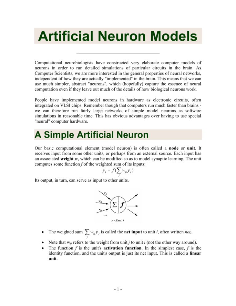
Artificial Neuron Models
Computational neurobiologists have constructed very elaborate computer models of
neurons in order to run detailed simulations of particular circuits in the brain. As
Computer Scientists, we are more interested in the general properties of neural networks,
independent of how they are actually "implemented" in the brain. This means that we can
use much simpler, abstract "neurons", which (hopefully) capture the essence of neural
computation even if they leave out much of the details of how biological neurons work.
People have implemented model neurons in hardware as electronic circuits, often
integrated on VLSI chips. Remember though that computers run much faster than brains we can therefore run fairly large networks of simple model neurons as software
simulations in reasonable time. This has obvious advantages over having to use special
"neural" computer hardware.
A Simple Artificial Neuron
Our basic computational element (model neuron) is often called a node or unit. It
receives input from some other units, or perhaps from an external source. Each input has
an associated weight w, which can be modified so as to model synaptic learning. The unit
computes some function f of the weighted sum of its inputs:
y i  f ( wij y j )
j
Its output, in turn, can serve as input to other units.

The weighted sum
w
ij
y j is called the net input to unit i, often written neti.
j


Note that wij refers to the weight from unit j to unit i (not the other way around).
The function f is the unit's activation function. In the simplest case, f is the
identity function, and the unit's output is just its net input. This is called a linear
unit.
-1-
Linear Regression
Fitting a Model to Data
Consider the data below (for more complete auto data, see data description, raw data, and
maple plots):
(Fig. 1)
Each dot in the figure provides information about the weight (x-axis, units: U.S. pounds)
and fuel consumption (y-axis, units: miles per gallon) for one of 74 cars (data from
1979). Clearly weight and fuel consumption are linked, so that, in general, heavier cars
use more fuel.
Now suppose we are given the weight of a 75th car, and asked to predict how much fuel
it will use, based on the above data. Such questions can be answered by using a model - a
short mathematical description - of the data (see also optical illusions). The simplest
useful model here is of the form
y = w1 x + w0
(1)
This is a linear model: in an xy-plot, equation 1 describes a straight line with slope w1
and intercept w0 with the y-axis, as shown in Fig. 2. (Note that we have rescaled the
coordinate axes - this does not change the problem in any fundamental way.)
How do we choose the two parameters w0 and w1 of our model? Clearly, any straight line
drawn somehow through the data could be used as a predictor, but some lines will do a
better job than others. The line in Fig. 2 is certainly not a good model: for most cars, it
will predict too much fuel consumption for a given weight.
-2-
(Fig. 2)
The Loss Function
In order to make precise what we mean by being a "good predictor", we define a loss
(also called objective or error) function E over the model parameters. A popular choice
for E is the sum-squared error:
(2)
In words, it is the sum over all points i in our data set of the squared difference between
the target value ti (here: actual fuel consumption) and the model's prediction yi,
calculated from the input value xi (here: weight of the car) by equation 1. For a linear
model, the sum-sqaured error is a quadratic function of the model parameters. Figure 3
shows E for a range of values of w0 and w1. Figure 4 shows the same functions as a
contour plot.
(Fig. 3)
(Fig. 4)
-3-
Minimizing the Loss
The loss function E provides us with an objective measure of predictive error for a
specific choice of model parameters. We can thus restate our goal of finding the best
(linear) model as finding the values for the model parameters that minimize E.
For linear models, linear regression provides a direct way to compute these optimal
model parameters. (See any statistics textbook for details.) However, this analytical
approach does not generalize to nonlinear models (which we will get to by the end of
this lecture). Even though the solution cannot be calculated explicitly in that case, the
problem can still be solved by an iterative numerical technique called gradient descent.
It works as follows:
1. Choose some (random) initial values for the model parameters.
2. Calculate the gradient G of the error function with respect to each model
parameter.
3. Change the model parameters so that we move a short distance in the direction of
the greatest rate of decrease of the error, i.e., in the direction of -G.
4. Repeat steps 2 and 3 until G gets close to zero.
How does this work? The gradient of E gives us the direction in which the loss function
at the current settting of the w has the steepest slope. In order to decrease E, we take a
small step in the opposite direction, -G (Fig. 5).
(Fig. 5)
By repeating this over and over, we move "downhill" in E until we reach a minimum,
where G = 0, so that no further progress is possible (Fig. 6).
(Fig. 6)
Fig. 7 shows the best linear model for our car data, found by this procedure.
-4-
(Fig. 7)
It's a neural network!
Our linear model of equation 1 can in fact be implemented by the simple neural network
shown in Fig. 8. It consists of a bias unit, an input unit, and a linear output unit. The
input unit makes external input x (here: the weight of a car) available to the network,
while the bias unit always has a constant output of 1. The output unit computes the sum:
y2 = y1 w21 + 1.0 w20
(3)
It is easy to see that this is equivalent to equation 1, with w21 implementing the slope of
the straight line, and w20 its intercept with the y-axis.
(Fig. 8)
Linear Neural Networks
Multiple regression
Our car example showed how we could discover an optimal linear function for predicting
one variable (fuel consumption) from one other (weight). Suppose now that we are also
given one or more additional variables which could be useful as predictors. Our simple
-5-
neural network model can easily be extended to this case by adding more input units (Fig.
1).
Similarly, we may want to predict more than one variable from the data that we're given.
This can easily be accommodated by adding more output units (Fig. 2). The loss function
for a network with multiple outputs is obtained simply by adding the loss for each output
unit together. The network now has a typical layered structure: a layer of input units (and
the bias), connected by a layer of weights to a layer of output units.
(Fig. 1)
(Fig. 2)
Computing the gradient
In order to train neural networks such as the ones shown above by gradient descent, we
need to be able to compute the gradient G of the loss function with respect to each weight
wij of the network. It tells us how a small change in that weight will affect the overall
error E. We begin by splitting the loss function into separate terms for each point p in the
training data:
(1)
where o ranges over the output units of the network. (Note that we use the superscript p
to denote the training point - this is not an exponentiation!) Since differentiation and
summation are interchangeable, we can likewise split the gradient into separate
components for each training point:
(2)
In what follows, we describe the computation of the gradient for a single data point,
omitting the superscript p in order to make the notation easier to follow.
First use the chain rule to decompose the gradient into two factors:
-6-
(3)
The first factor can be obtained by differentiating Eqn. 1 above:
(4)
Using y o   woj y j , the second factor becomes
j
(5)
Putting the pieces (equations 3-5) back together, we obtain
(6)
To find the gradient G for the entire data set, we sum at each weight the contribution
given by equation 6 over all the data points. We can then subtract a small proportion µ
(called the learning rate) of G from the weights to perform gradient descent.
The Gradient Descent Algorithm
1. Initialize all weights to small random values.
2. REPEAT until done
1. For each weight wij set wij : 0
2. For each data point (x, t)p
1. set input units to x
2. compute value of output units
3. For each weight wij set wij : wij  (t i  y i ) y j
3. For each weight wij set wij : wij  wij
The algorithm terminates once we are at, or sufficiently near to, the minimum of the error
function, where G = 0. We say then that the algorithm has converged.
The Learning Rate
-7-
An important consideration is the learning rate µ, which determines by how much we
change the weights w at each step. If µ is too small, the algorithm will take a long time to
converge (Fig. 3).
(Fig. 3)
(Fig. 4)
Conversely, if µ is too large, we may end up bouncing around the error surface out of
control - the algorithm diverges (Fig. 4). This usually ends with an overflow error in the
computer's floating-point arithmetic.
Multi-layer networks
A nonlinear problem
Consider again the best linear fit we found for the car data. Notice that the data points are
not evenly distributed around the line: for low weights, we see more miles per gallon than
our model predicts. In fact, it looks as if a simple curve might fit these data better than
the straight line. We can enable our neural network to do such curve fitting by giving it
an additional node which has a suitably curved (nonlinear) activation function. A useful
function for this purpose is the S-shaped hyperbolic tangent (tanh) function (Fig. 1).
(Fig. 1)
(Fig. 2)
Fig. 2 shows our new network: an extra node (unit 2) with tanh activation function has
been inserted between input and output. Since such a node is "hidden" inside the network,
-8-
it is commonly called a hidden unit. Note that the hidden unit also has a weight from the
bias unit. In general, all non-input neural network units have such a bias weight. For
simplicity, the bias unit and weights are usually omitted from neural network diagrams unless it's explicitly stated otherwise, you should always assume that they are there.
(Fig. 3)
When this network is trained by gradient descent on the car data, it learns to fit the tanh
function to the data (Fig. 3). Each of the four weights in the network plays a particular
role in this process: the two bias weights shift the tanh function in the x- and y-direction,
respectively, while the other two weights scale it along those two directions. Fig. 2 gives
the weight values that produced the solution shown in Fig. 3.
Hidden Layers
One can argue that in the example above we have cheated by picking a hidden unit
activation function that could fit the data well. What would we do if the data looks like
this (Fig. 4)?
(Fig. 4)
(Relative concentration of NO and NO2 in exhaust fumes as a function
of the richness of the ethanol/air mixture burned in a car engine.)
Obviously the tanh function can't fit this data at all. We could cook up a special activation
function for each data set we encounter, but that would defeat our purpose of learning to
model the data. We would like to have a general, non-linear function approximation
method which would allow us to fit any given data set, no matter how it looks like.
-9-
(Fig. 5)
Fortunately there is a very simple solution: add more hidden units! In fact, a network with
just two hidden units using the tanh function (Fig. 5) can fit the data in Fig. 4 quite well can you see how? The fit can be further improved by adding yet more units to the hidden
layer. Note, however, that having too large a hidden layer - or too many hidden layers can degrade the network's performance (more on this later). In general, one shouldn't use
more hidden units than necessary to solve a given problem. (One way to ensure this is to
start training with a very small network. If gradient descent fails to find a satisfactory
solution, grow the network by adding a hidden unit, and repeat.)
Theoretical results indicate that given enough hidden units, a network like the one in Fig.
5 can approximate any reasonable function to any required degree of accuracy. In other
words, any function can be expressed as a linear combination of tanh functions: tanh is a
universal basis function. Many functions form a universal basis; the two classes of
activation functions commonly used in neural networks are the sigmoidal (S-shaped)
basis functions (to which tanh belongs), and the radial basis functions.
Error Backpropagation
We have already seen how to train linear networks by gradient descent. In trying to do
the same for multi-layer networks we encounter a difficulty: we don't have any target
values for the hidden units. This seems to be an insurmountable problem - how could we
tell the hidden units just what to do? This unsolved question was in fact the reason why
neural networks fell out of favor after an initial period of high popularity in the 1950s. It
took 30 years before the error backpropagation (or in short: backprop) algorithm
popularized a way to train hidden units, leading to a new wave of neural network research
and applications.
(Fig. 1)
In principle, backprop provides a way to train networks with any number of hidden units
arranged in any number of layers. (There are clear practical limits, which we will discuss
- 10 -
later.) In fact, the network does not have to be organized in layers - any pattern of
connectivity that permits a partial ordering of the nodes from input to output is allowed.
In other words, there must be a way to order the units such that all connections go from
"earlier" (closer to the input) to "later" ones (closer to the output). This is equivalent to
stating that their connection pattern must not contain any cycles. Networks that respect
this constraint are called feedforward networks; their connection pattern forms a
directed acyclic graph or dag.
The Algorithm
We want to train a multi-layer feedforward network by gradient descent to approximate
an unknown function, based on some training data consisting of pairs (x,t). The vector x
represents a pattern of input to the network, and the vector t the corresponding target
(desired output). As we have seen before, the overall gradient with respect to the entire
training set is just the sum of the gradients for each pattern; in what follows we will
therefore describe how to compute the gradient for just a single training pattern. As
before, we will number the units, and denote the weight from unit j to unit i by wij.
1. Definitions:
o
the error signal for unit j:
o
the (negative) gradient for weight wij:
o
the set of nodes anterior to unit i:
o
the set of nodes posterior to unit j:
2. The gradient. As we did for linear networks before, we expand the gradient into
two factors by use of the chain rule:
The first factor is the error of unit i. The second is
Putting the two together, we get
.
To compute this gradient, we thus need to know the activity and the error for all
relevant nodes in the network.
3. Forward activation. The activity of the input units is determined by the
network's external input x. For all other units, the activity is propagated forward:
- 11 -
Note that before the activity of unit i can be calculated, the activity of all its anterior
nodes (forming the set Ai) must be known. Since feedforward networks do not contain
cycles, there is an ordering of nodes from input to output that respects this condition.
4. Calculating output error. Assuming that we are using the sum-squared loss
the error for output unit o is simply
5. Error backpropagation. For hidden units, we must propagate the error back
from the output nodes (hence the name of the algorithm). Again using the chain
rule, we can expand the error of a hidden unit in terms of its posterior nodes:
Of the three factors inside the sum, the first is just the error of node i. The second
is
while the third is the derivative of node j's activation function:
For hidden units h that use the tanh activation function, we can make use of the
special identity tanh(u)' = 1 - tanh(u)2, giving us
Putting all the pieces together we get
Note that in order to calculate the error for unit j, we must first know the error of all its
posterior nodes (forming the set Pj). Again, as long as there are no cycles in the network,
there is an ordering of nodes from the output back to the input that respects this
condition. For example, we can simply use the reverse of the order in which activity was
propagated forward.
Matrix Form
For layered feedforward networks that are fully connected - that is, each node in a given
layer connects to every node in the next layer - it is often more convenient to write the
backprop algorithm in matrix notation rather than using more general graph form given
above. In this notation, the biases weights, net inputs, activations, and error signals for all
- 12 -
units in a layer are combined into vectors, while all the non-bias weights from one layer
to the next form a matrix W. Layers are numbered from 0 (the input layer) to L (the
output layer). The backprop algorithm then looks as follows:
1. Initialize the input layer:
2. Propagate activity forward: for l = 1, 2, ..., L,
where bl is the vector of bias weights.
3. Calculate the error in the output layer:
4. Backpropagate the error: for l = L-1, L-2, ..., 1,
where T is the matrix transposition operator.
5. Update the weights and biases:
You can see that this notation is significantly more compact than the graph form, even
though it describes exactly the same sequence of operations.
Backpropagation of
error: an example
We will now show an example of a backprop network as it learns to model the highly
nonlinear data we encountered before.
- 13 -
The left hand panel shows the data to be modeled. The right hand panel shows a network
with two hidden units, each with a tanh nonlinear activation function. The output unit
computes a linear combination of the two functions
yo  f tanh 1( x)  g tanh 2( x)  a
(1)
Where
tanh 1( x)  tanh( dx  b)
(2)
and
tanh 2( x)  tanh( ex  c)
(3)
To begin with, we set the weights, a..g, to random initial values in the range [-1,1]. Each
hidden unit is thus computing a random tanh function. The next figure shows the initial
two activation functions and the output of the network, which is their sum plus a negative
constant. (If you have difficulty making out the line types, the top two curves are the tanh
functions, the one at the bottom is the network output).
As the activation functions are stretched, scaled and shifted by the changing weights, we
hope that the error of the model is dropping. In the next figure we plot the total sum
squared error over all 88 patterns of the data as a function of training epoch. Four training
runs are shown, with different weight initialization each time:
By
Genevieve
Orr,
of
Willamette
University,
http://www.willamette.edu/~gorr/classes/cs449/intro.html
- 14 -
found
at