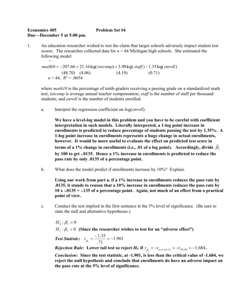
Economics 405
Due—December 5 at 5:00 pm.
1.
Problem Set #4
An education researcher wished to test the claim that larger schools adversely impact student test
scores. The researcher collected data for n = 44 Michigan high schools. She estimated the
following model
^
math10  207.66  21.16 log( totcomp)  3.98 log( staff )  1.35 log( enroll )
(48.70) (4.06)
(4.19)
(0.71)
2
n = 44, R = .0654
where math10 is the percentage of tenth-graders receiving a passing grade on a standardized math
test; totcomp is average annual teacher compensation; staff is the number of staff per thousand
students; and enroll is the number of students enrolled.
a.
Interpret the regression coefficient on log(enroll).
We have a level-log model in this problem and you have to be careful with coefficient
interpretation in such models. Literally interpreted, a 1-log point increase in
enrollments is predicted to reduce percentage of students passing the test by 1.35%. A
1-log point increase in enrollments represents a huge change in actual enrollments,
however. It would be more useful to evaluate the effect on predicted test score in
terms of a 1% change in enrollments (i.e., .01 of a log point). Accordingly, divide ̂ 3
by 100 to get -.0135. Hence a 1% increase in enrollments is predicted to reduce the
pass rate by only .0135 of a percentage point.
b.
What does the model predict if enrollments increase by 10%? Explain.
Using our work from part a, if a 1% increase in enrollments reduces the pass rate by
.0135, it stands to reason that a 10% increase in enrollments reduces the pass rate by
10 x -.0135 = -.135 of a percentage point. Again, not much of an effect from a practical
point of view.
c.
Conduct the test implied in the first sentence at the 5% level of significance. (Be sure to
state the null and alternative hypotheses.)
H 0 : 3  0
H 1 :  3  0 (Since the researcher wishes to test for an “adverse effect”)
 1.35
 1.901
Test Statistic: t ˆ 
3
.71
Rejection Rule: Lower tail test so reject H0 if t ˆ  t ,n( k 1)  t.05, 40  1.684 .
3
Conclusion: Since the test statistic, at -1.901, is less than the critical value of -1.684, we
reject the null hypothesis and conclude that enrollments do have an adverse impact on
the pass rate at the 5% level of significance.
2
d.
Would the conclusion to part c change if the 1% level of significance were used? Why or
why not?
 t.01, 40  2.423 , therefore the test statistic would not be in the rejection region if we
use the 1% significance level. So the evidence against the null hypothesis of no effect is
strong but not the strongest possible evidence.
e.
Use Excel to generate the p-value of the test statistic. Explain how you obtained the pvalue. Interpret the p-value obtained for the test statistic in this problem.
Use the TDIST function with X = 1.901, degrees of freedom = 40, and one tail.
Using Excel, it turns out that the p-value for t ˆ  1.901 is .032. Note that this is
3
between .05 and .01, which explains why we can reject at the 5% level but not at the
1% level. p-value equal .032 implies that if the null hypothesis is correct, there is a
3.2% chance of randomly sampling 44 schools and obtaining ˆ3  1.35 . In other
words, there’s not much chance of getting the result we got if enrollments really don’t
affect the pass rate.
3
2.
The RENTAL.dta dataset from Wooldridge contains information on rent in college towns. I
regressed log(rent) on log(pop), log(avginc), and pctstu, where rent is average monthly rent, pop is
total town population, avginc is average household income, and pctstu is the percentage of students
in the total town population. Here is the regression output:
Source |
SS
df
MS
-------------+-----------------------------Model | 11.2058779
3 3.73529263
Residual | 2.85225674
124
.02300207
-------------+-----------------------------Total | 14.0581346
127 .110693974
Number of obs
F( 3,
124)
Prob > F
R-squared
Adj R-squared
Root MSE
=
=
=
=
=
=
128
162.39
0.0000
0.7971
0.7922
.15166
---------------------------------------------------------lrent |
Coef.
Std. Err.
t
P>|t|
-------------+-------------------------------------------lpop |
.0313456
.0270786
1.16
0.249
lavginc |
.8771387
.0413247
21.23
0.000
pctstu |
.0065849
.0012027
5.48
0.000
_cons | -3.368309
.4639438
-7.26
0.000
---------------------------------------------------------
a.
Interpret the regression coefficient on lavginc.
Since both the dependent variable and the independent variable of interest are in logs,
the coefficient on lavginc is the estimated elasticity of rent with respect to average
community income. Given ˆlavginc  .877 , our interpretation would be that a 1%
increase in the average income of a community results in a .877 of a percent increase in
average rent, holding log population and the percent of students equal across
communities. Alternatively, it would also be correct to say that a 10% increase in
average community income leads to an 8.77% increase in average rents, other things
equal.
b.
Using an   .05 , test the null hypothesis that the elasticity of rents with respect to income
equals 1 against the lower-tail alternative. In conducting the test, write out the null
hypothesis, the alternative hypothesis, the test statistic, the rejection region, and the
conclusion.
H 0 :  lavginc  1
H 1 :  lavginc  1
Rejection Region: Reject H0 if t ˆlavg inc  t.05,124  1.658 .
Test Statistic: t ˆ
lavginc

ˆlavginc  1
se( ˆ
lavginc
)

.877  1
 3
.041
Since the test statistic is less than the critical value, we should reject the null hypothesis
of unitary elasticity with respect to income. In other words, we can conclude that
while student rents rise with community income they do not do so proportionately.
4
c.
Use Excel to generate the p-value of the test statistic. Explain how you obtained the pvalue. Interpret the p-value obtained for the test statistic in this problem.
Use TDIST in excel, setting X = 3, degrees of freedom = 124, tails = 1.
The p-value equals .0016. Since the p-value is less than even   .01, we conclude that
the test statistic is highly significant. Specifically, there is less than a 2/10 of 1%
chance in repeated sampling of obtaining an estimated regression coefficient of .877 or
less when the null hypothesis of unitary elasticity is actually true. Essentially, there’s
no way that the elasticity of rents with respect to income is equal to one given the
sample evidence.
3.
Consider the population model: y   0  1 x1   2 x2   3 x3   4 x4   5 x5  u . There is
some question as to whether x4 and x5 belong in the model at all. Neither x4 nor x5 was
statistically significant in the estimated unrestricted regression. Conduct a test to
determine whether x4 and x5 are jointly significant at the 10% level. The sample size is n
= 32. The SSR of the restricted model is SSRr  3,047 and the SSR of the unrestricted
model is SSRur  2,691 .
a.
What is the null hypothesis? Explain.
The question is whether x4 and x5 should be in the model at all. The null
hypothesis, then, imposes q = 2 exclusion restrictions on the model, such that
H 0 :  4  0, 5  0 .
5
b.
What is the alternative hypothesis? Explain.
The alternative hypothesis in a test of joint significance is that the null
hypothesis is not true. This allows for the possibility in the problem at hand
that either x4 has an effect on the dependent variable, that x5 has an effect on
the dependent variable, or that both x4 and x5 have an effect on the
dependent variable. Formally,
H 1 : H 0 is not true
c.
Calculate the test statistic. Show your work.
We know the restricted and unrestricted residual sums of squares and we
know that n = 32, k = 5, and q = 2. The appropriate test statistic is:
F
d.
( SSRr  SSRur ) / q
(3,047  2,691) / 2
178


 1.7198
SSRur /( n  (k  1)) 2,691 /(32  (5  1)) 103.5
What is the critical value for the test statistic? Explain/show.
The F-statistic is distributed as an F random variable with q numerator
degrees of freedom and n-(k+1) denominator degrees of freedom under the
null hypothesis. The test for joint significance is strictly an upper tail test.
The desired level of significance is   .10 , i.e., the weakest level of evidence.
Notice that I don’t set the significance level at .05 or .01. We’re looking for
any evidence that variation in x4 and/or x5 explain some of the variation in y.
If we find even weak evidence, we should retain the variables in the
regression, otherwise we’re likely to induce omitted variable bias. We would
rather accept some inefficiency in the coefficient standard errors than cause
bias in the coefficient estimates of the remaining included regressors.
We’ll reject the null hypothesis if
F  F ,q ,n ( k 1)  F.10, 2, 26  2.52 .
e.
Are x4 and x5 jointly significant? Why or why not?
Since F = 1.7198, the test statistic does not satisfy the rejection rule. Hence
we cannot reject the null hypothesis that x4 and x5 have no effect on the
dependent variable at even the 10% level of significance. It would seem there
would be no harm in excluding these regressors from the model.
Furthermore, we should gain some precision in the estimation of the effects
of x1 – x3, since exclusion of x4 and x5 should reduce the degree of collinearity
amongst the remaining regressors.
6
f.
Use Excel to generate the p-value of the test statistic. Explain how you obtained
the p-value. Interpret the p-value of the test statistic.
Use FDIST setting X = 1.7198, Deg_freedom1 = 2, and Deg_freedom2 = 26.
The resulting p-value is .199. In other words, the probability is almost 20%
of getting a test statistic at least as large as 1.7198 when the null hypothesis of
no effect from x4 and x5 is true. This p-value is greater than all conventional
significance levels and so we cannot reject the null hypothesis at any of the
conventional significance levels (of course, this fact is clear in part e, since we
couldn’t reject H 0 at even the .10 level of significance there).