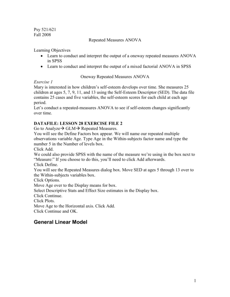
Psy 521/621
Fall 2008
Repeated Measures ANOVA
Learning Objectives
 Learn to conduct and interpret the output of a oneway repeated measures ANOVA
in SPSS
 Learn to conduct and interpret the output of a mixed factorial ANOVA in SPSS
Oneway Repeated Measures ANOVA
Exercise 1
Mary is interested in how children’s self-esteem develops over time. She measures 25
children at ages 5, 7, 9, 11, and 13 using the Self-Esteem Descriptor (SED). The data file
contains 25 cases and five variables, the self-esteem scores for each child at each age
period.
Let’s conduct a repeated-measures ANOVA to see if self-esteem changes significantly
over time.
DATAFILE: LESSON 28 EXERCISE FILE 2
Go to Analyze GLM Repeated Measures.
You will see the Define Factors box appear. We will name our repeated multiple
observations variable Age. Type Age in the Within-subjects factor name and type the
number 5 in the Number of levels box.
Click Add.
We could also provide SPSS with the name of the measure we’re using in the box next to
“Measure:” If you choose to do this, you’ll need to click Add afterwards.
Click Define.
You will see the Repeated Measures dialog box. Move SED at ages 5 through 13 over to
the Within-subjects variables box.
Click Options.
Move Age over to the Display means for box.
Select Descriptive Stats and Effect Size estimates in the Display box.
Click Continue.
Click Plots.
Move Age to the Horizontal axis. Click Add.
Click Continue and OK.
General Linear Model
1
Within-Subjects Factors
Measure: MEASURE_1
Dependent
Variable
sed1
sed2
sed3
sed4
sed5
age
1
2
3
4
5
De scriptive Statistics
Self-es teem
Self es teem
Self-es teem
Self-es teem
Self-es teem
at
at
at
at
at
age
age
age
age
age
5
7
9
11
13
Mean
33.88
27.60
29.60
29.96
16.08
St d. Deviation
27.917
35.352
31.492
34.863
16.951
N
25
25
25
25
25
Multivaria te Testsb
Effect
age
Pillai's Trac e
W ilks' Lambda
Hotelling's Trac e
Roy's Largest Root
Value
.555
.445
1.247
1.247
F
Hy pothesis df
6.549a
4.000
6.549a
4.000
a
6.549
4.000
6.549a
4.000
Error df
21.000
21.000
21.000
21.000
Sig.
.001
.001
.001
.001
Partial Eta
Squared
.555
.555
.555
.555
a. Ex act statistic
b.
Design: Int ercept
W ithin Subject s Design: age
b
Ma uchly's Test of Spheri city
Measure: MEA SURE_1
a
Epsilon
W ithin Subject s Effect Mauchly's W
age
.470
Approx .
Chi-Square
16.945
df
9
Sig.
.050
Greenhous
e-Geis ser
.747
Huynh-Feldt
.865
Lower-bound
.250
Tests the null hypothes is that t he error covariance matrix of the orthonormalized transformed dependent variables is
proportional to an ident ity matrix.
a. May be us ed t o adjust the degrees of freedom for the averaged t ests of s ignificance. Corrected tests are displayed in
the Tests of W ithin-Subject s Effect s table.
b.
Design: Int ercept
W ithin Subject s Design: age
2
Tests of Within-Subjects Effects
Measure: MEASURE_1
Source
age
Error(age)
Type III Sum
of Squares
4539.088
4539.088
4539.088
4539.088
22834.512
22834.512
22834.512
22834.512
Sphericity Assumed
Greenhous e-Geisser
Huynh-Feldt
Lower-bound
Sphericity Assumed
Greenhous e-Geisser
Huynh-Feldt
Lower-bound
df
4
2.989
3.461
1.000
96
71.727
83.058
24.000
Mean Square
1134.772
1518.796
1311.589
4539.088
237.859
318.355
274.922
951.438
F
4.771
4.771
4.771
4.771
Sig.
.001
.004
.003
.039
Partial Eta
Squared
.166
.166
.166
.166
Te sts of Betwe en-Subjects Effects
Measure: MEASURE_1
Transformed Variable: Average
Source
Int ercept
Error
Ty pe III Sum
of Squares
94009. 472
85732. 928
df
1
24
Mean Square
94009. 472
3572.205
F
26.317
Sig.
.000
Partial Eta
Squared
.523
Estimated Marginal Means
age
Measure: MEASURE_1
age
1
2
3
4
5
Mean
33.880
27.600
29.600
29.960
16.080
Std. Error
5.583
7.070
6.298
6.973
3.390
95% Confidence Interval
Lower Bound Upper Bound
22.356
45.404
13.007
42.193
16.601
42.599
15.569
44.351
9.083
23.077
Profile Plots
Estimated Marginal Means of MEASURE_1
Estimated Marginal Means
35
30
25
20
15
1
2
3
4
5
age
As the omnibus ANOVA is significant, we will conduct two types of follow-up tests:
1) a polynomial contrast: set as a default in SPSS, so we don’t have to ask for them
3
*Note: polynomial contrasts are most appropriate when the variable is continuous
in nature (e.g., time).
2) a Fisher’s LSD test: Click Options, move “age” into the “Display means for” window
and below that window check the box next to “compare main effects.” LSD is the default,
but you can use the drop down menu to see what your other options are (i.e., Bonferroni
& Sidak)
*Note: we will run these contrasts for pedagogical purposes, but interpretation of
the contrasts are more meaningful since the variable (age) is truly continuous
Tests of Within-Subjects Contrasts
Measure: MEASURE_1
Source
age
Error(age)
age
Linear
Quadratic
Cubic
Order 4
Linear
Quadratic
Cubic
Order 4
Type III Sum
of Squares
2762.244
506.403
1267.876
2.565
6235.456
9469.383
2524.424
4605.249
df
1
1
1
1
24
24
24
24
Mean Square
2762.244
506.403
1267.876
2.565
259.811
394.558
105.184
191.885
F
10.632
1.283
12.054
.013
Sig.
.003
.268
.002
.909
Partial Eta
Squared
.307
.051
.334
.001
(see Howell p. 677 for the polynomial coefficients)
4
Pairwise Comparisons
Measure: MEASURE_1
(I) age
1
2
3
4
5
(J) age
2
3
4
5
1
3
4
5
1
2
4
5
1
2
3
5
1
2
3
4
Mean
Difference
(I-J)
6.280
4.280
3.920
17.800*
-6.280
-2.000
-2.360
11.520*
-4.280
2.000
-.360
13.520*
-3.920
2.360
.360
13.880*
-17.800*
-11.520*
-13.520*
-13.880*
Std. Error
3.662
4.574
4.509
4.148
3.662
3.827
3.464
5.533
4.574
3.827
3.513
4.780
4.509
3.464
3.513
5.097
4.148
5.533
4.780
5.097
a
Sig.
.099
.359
.393
.000
.099
.606
.502
.048
.359
.606
.919
.009
.393
.502
.919
.012
.000
.048
.009
.012
95% Confidence Interval for
a
Difference
Lower Bound Upper Bound
-1.278
13.838
-5.160
13.720
-5.387
13.227
9.240
26.360
-13.838
1.278
-9.898
5.898
-9.508
4.788
.101
22.939
-13.720
5.160
-5.898
9.898
-7.611
6.891
3.655
23.385
-13.227
5.387
-4.788
9.508
-6.891
7.611
3.361
24.399
-26.360
-9.240
-22.939
-.101
-23.385
-3.655
-24.399
-3.361
Based on estimated marginal means
*. The mean difference is s ignificant at the .05 level.
a. Adjustment for multiple comparisons: Leas t Significant Difference (equivalent to no
adjustments).
We can see from the post hoc analyses that self-esteem at age thirteen is significantly
lower than self-esteem at ages 5, 7, 9, and 11. Ages 5, 7, 9, and 11 do not differ from one
another is a systematic manner.
APA results:
A one-way within-subjects analysis of variance was conducted to determine
whether self-esteem changes significantly as children develop. The factor, age, had five
levels (5, 7, 9, 11, and 13), the dependent variable was scores on the Self-Esteem
Descriptor (SED) with higher scores indicating higher self-esteem. Twenty-five children
participated in the study over eight years. Mauchly’s test was significant, therefore
sphericity was not assumed and the Greenhouse-Geisser correction was employed. The
results indicate a significant age effect on self-esteem, F(3, 72) = 4.77, p < .05, partial η2
= .17.
Follow-up polynomial contrasts indicate significant linear and cubic trends, F(1,
24) = 10.63, p = .003, partial η2= .31 and F(1, 24) = 12.05, p < .05, partial η2= .33,
5
respectively. [The linear trend suggests that mean self-esteem scores decrease with age: 5
(M = 33.88, SD = 27.92), 7 (M = 27.60, SD = 35.35), 9 (M = 29.60, SD = 31.49), 11 (M =
29.96, SD = 34.86), and 13 (M = 16.08, SD = 16.95). The cubic trend suggests that selfesteem at age 5 is the highest and self-esteem at age 13 is the lowest, while self-esteem at
ages 7, 9, and 11 is moderate and does not change across this intermediate time period.
FYI: if you were comparing treatment types (i.e., categories) rather than trends in
age or time, you would report post hoc analyses. Below is an example of the followup portion of the APA section for a post hoc situation.
Follow-up post hoc analyses were conducted using Fisher’s LSD. The results
indicate that average self-esteem scores at age 13 (M = 16.08, SD = 16.95) are
significantly lower than average self-esteem scores at ages 5 (M = 33.88, SD = 27.92), 7
(M = 27.60, SD = 35.35), 9 (M = 29.60, SD = 31.49), and 11 (M = 29.96, SD = 34.86).
Self-esteem at ages 5, 7, 9, and 11 did not differ from one another is a systematic manner.
Mixed Factorial ANOVA
Exercise 2
A researcher wants to study a phenomenon in memory and learning research called
proactive interference. Proactive interference occurs when you attempt to learn new
information and previously learned information interferes with the new material. For the
experiment, the researcher had the participants complete a series of trials. On each trial,
the researcher presented the participant with a short list of words whose meanings are
highly related (e.g., names of flowers). After seeing the words, the participant then had
to recall the words in the list. For the experimental and control groups, to which
participants were randomly assigned, the first three trials used the same category of
words. On the fourth trial, the researcher changed the meaning of the words for the
experimental group (e.g., names of professions rather than names of flowers), but left the
meaning of the words for the control group unchanged.
Do we understand why this is a mixed factorial design? What is the within subjects
factor? Trials: it is a within subjects factor because each participant participates in every
trial. What is the between subjects factor? Experimental group (experimental or control)
is the between subjects factor because a participants are in either the experimental or
control group, not both.
Let’s draw out, conceptually, how we are going to partition the variance in this model:
TOTAL
VARIATION
Between subjects
Group (G)
Errorbetween
(SS w/in groups)
Within subjects
Trial (T)
TXG
Errorwithin
(T X SS w/in groups)
6
Let’s conduct a mixed factorial ANOVA to see if differences in scores across trials differ
for the experimental group vs. the control group (i.e., depending on experimental
condition).
DATAFILE: PROACTIVE.SAV
Go to Analyze GLM Repeated Measures.
You will see the Define Factors box appear. We will name our repeated multiple
observations variable Trial. Type Trial in the Within-subjects factor name and type the
number 4 in the Number of levels box. Why do we enter a 4 here?
Click Add.
Click Define. You will see the Repeated Measures dialog box. Move trial 1 through 4
over to the Within-subjects variables box. Move Group to the Between-subjects factors
box.
Click Options. Move group, trial, and group*trial over to the Display means for box.
Select Descriptive Stats, Effect Size estimates, and Homogeneity test in the Display box.
Click Continue.
Click Plots. Move Trial to the Horizontal axis and Group to the Separate lines box. Click
Add.
Click Continue and OK.
Even though this info shows up near the end in the output, let’s look at the plot we
created first to get a visual understanding of what’s happening with our data.
Profile Plots
Estimated Marginal Means of MEASURE_1
Experimental
Condition
80.00
Experimental
Estimated Marginal Means
Control
70.00
60.00
50.00
40.00
30.00
1
2
3
4
trial
7
Our between subjects factor (group) is being represented by the lines (blue for exp. green
for control). Our within subjects factor is represented on the horizontal axis. What seems
to be happening?
Let’s think first in terms of main effects:
Trial: It seems as though participant memory is declining across trials, although
(averaging across conditions) it seems to turn upward a bit on Trial 4. To get an idea of
this main effect we are looking at the average of the two groups at each trial (e.g.,
average the two dots for Trial 1, average the two dots for Trial 2, etc, then compare the 4
values. If they are the same, the main effect for trial is probably not significant).
Group: Probably not a main effect here, but it is a little difficult to tell from the graph. To
get an idea of this main effect we are comparing the average memory score across trials
for each group (e.g., create an average of all of the dots on the blue line, create an average
of all the dots on the green line, then compare the two. If they are the same, the main
effect for group is probably not significant)
Would you guess that there is a group X trial interaction? Likely so because of the
relatively extreme differences in the values for the exp. vs. control groups in the 4th trial.
General Linear Model
Within-Subjects Factors
Measure: MEASURE_1
trial
1
2
3
4
Dependent
Variable
trial1
trial2
trial3
trial4
Between-Subjects Factors
Experimental
Condition
1.00
2.00
Value Label
Experiment
al
Control
N
5
5
8
Descriptive Statistics
Trial 1 Memory
Trial 2 Memory
Trial 3 Memory
Trial 4 Memory
Experimental Condition
Experimental
Control
Total
Experimental
Control
Total
Experimental
Control
Total
Experimental
Control
Total
Mean
78.0000
77.2000
77.6000
50.2000
58.6000
54.4000
38.2000
43.2000
40.7000
64.8000
35.8000
50.3000
Std. Deviation
10.55936
8.81476
9.17969
5.93296
11.92896
9.92416
16.42255
8.16701
12.50822
9.88433
9.31128
17.76420
N
5
5
10
5
5
10
5
5
10
5
5
10
a
Box's Test of Equality of Covaria nce Ma trice
s
Box's M
F
df1
df2
Sig.
20.805
.894
10
305.976
.539
Tests the null hypothes is that t he observed covariance
matric es of the dependent variables are equal acros s groups .
a.
Design: Int ercept+group
W ithin Subject s Design: trial
Multivaria te Testsb
Effect
trial
trial * group
Pillai's Trac e
W ilks' Lambda
Hotelling's Trac e
Roy's Largest Root
Pillai's Trac e
W ilks' Lambda
Hotelling's Trac e
Roy's Largest Root
Value
.922
.078
11.847
11.847
.811
.189
4.288
4.288
F
Hy pothesis df
23.694 a
3.000
23.694 a
3.000
23.694 a
3.000
23.694 a
3.000
8.575a
3.000
8.575a
3.000
8.575a
3.000
8.575a
3.000
Error df
6.000
6.000
6.000
6.000
6.000
6.000
6.000
6.000
Sig.
.001
.001
.001
.001
.014
.014
.014
.014
Partial Eta
Squared
.922
.922
.922
.922
.811
.811
.811
.811
a. Ex act stat istic
b.
Design: Int ercept+group
W ithin Subject s Design: trial
9
b
Ma uchly's Test of Spheri city
Measure: MEA SURE_1
a
Epsilon
W ithin Subject s Effect Mauchly's W
trial
.856
Approx .
Chi-Square
1.045
df
5
Sig.
.959
Greenhous
e-Geis ser
.908
Huynh-Feldt
1.000
Lower-bound
.333
Tests the null hypothes is that t he error covariance matrix of the orthonormalized transformed dependent variables is
proportional to an ident ity matrix.
a. May be us ed t o adjust the degrees of freedom for the averaged t ests of s ignificance. Corrected tests are displayed in
the Tests of W ithin-Subject s Effect s table.
b.
Design: Int ercept+group
W ithin Subject s Design: trial
Mauchly’s test is ns, so we don’t have to worry about violating the sphericity assumption.
Te sts of W ithi n-Subje cts Effe cts
Measure: MEA SURE_1
Source
trial
trial * group
Error(t rial)
Sphericity Ass umed
Greenhous e-Geiss er
Huynh-Feldt
Lower-bound
Sphericity Ass umed
Greenhous e-Geiss er
Huynh-Feldt
Lower-bound
Sphericity Ass umed
Greenhous e-Geiss er
Huynh-Feldt
Lower-bound
Ty pe III Sum
of Squares
7354.500
7354.500
7354.500
7354.500
2174.900
2174.900
2174.900
2174.900
1952.600
1952.600
1952.600
1952.600
df
3
2.723
3.000
1.000
3
2.723
3.000
1.000
24
21.785
24.000
8.000
Mean Square
2451.500
2700.734
2451.500
7354.500
724.967
798.671
724.967
2174.900
81.358
89.630
81.358
244.075
F
30.132
30.132
30.132
30.132
8.911
8.911
8.911
8.911
Sig.
.000
.000
.000
.001
.000
.001
.000
.017
Partial Eta
Squared
.790
.790
.790
.790
.527
.527
.527
.527
Note that you have an error term here.
On the diagram on p. 451 this is referred
to as: “I x Ss w/in groups”
We have significant main effects for trial, and for the trialXgroup interaction. This is
what we suspected based on the plot.
10
Tests of Within-Subjects Contrasts
Measure: MEASURE_1
Source
trial
trial * group
Error(trial)
trial
Linear
Quadratic
Cubic
Linear
Quadratic
Cubic
Linear
Quadratic
Cubic
Type III Sum
of Squares
4569.680
2689.600
95.220
968.000
1166.400
40.500
451.720
887.000
613.880
df
1
1
1
1
1
1
8
8
8
Mean Square
4569.680
2689.600
95.220
968.000
1166.400
40.500
56.465
110.875
76.735
F
80.929
24.258
1.241
17.143
10.520
.528
Sig.
.000
.001
.298
.003
.012
.488
Partial Eta
Squared
.910
.752
.134
.682
.568
.062
Significant linear and quadratic trends exist for the trial main effect and the trialXgroup
interaction. This shouldn’t be surprising based on what we saw in the plot. In considering
the linear and quadratic trends for the main effect of trial, we saw that, averaging across
groups, scores tended to decline across trials (linear trend) until the 4th trial when there
was a slight improvement (quadratic trend). How do we interpret the significant linear
and quadratic trends for the trialXgroup interaction? Well, this basically means that the
linear/quadratic trend depends on the group you are in. Focusing on the significant linear
trend, it seems that the pattern displayed by the control group is driving the interaction,
i.e., the trend seems to be linear for the control group, but not the experimental group.
Now focusing on the significant quadratic trend, it seems that the pattern displayed by the
experimental group is driving, i.e., the trend is quadratic for the experimental group, but
not the control.
a
Le vene's Test of Equa lity of Error Va riances
Trial
Trial
Trial
Trial
1
2
3
4
Memory
Memory
Memory
Memory
F
.070
3.933
.987
.000
df1
df2
1
1
1
1
8
8
8
8
Sig.
.798
.083
.350
1.000
Tests the null hypothes is that t he error variance of the dependent
variable is equal ac ross groups.
a.
Design: Int ercept+group
W ithin Subject s Design: trial
11
Tests of Between-Subjects Effects
Measure: MEASURE_1
Transformed Variable: Average
Source
Intercept
group
Error
Type III Sum
of Squares
124322.500
168.100
1597.400
df
1
1
8
Mean Square
124322.500
168.100
199.675
F
622.624
.842
Sig.
.000
.386
Partial Eta
Squared
.987
.095
This is the main effect for group: as you can see it is ns. Again, this is what we
expected based on our plots.
And you have another error term here. On the diagram on p. 451 this is referred to as:
“Ss w/in groups.” So you now have TWO error terms: one for the within subjects effect,
and one for the between subjects effect.
Estimated Marginal Means
1. Experimental Condition
Measure: MEASURE_1
Experimental Condition
Experimental
Control
Mean
57.800
53.700
Std. Error
3.160
3.160
95% Confidence Interval
Lower Bound Upper Bound
50.514
65.086
46.414
60.986
2. trial
Measure: MEA SURE_1
trial
1
2
3
4
Mean
77.600
54.400
40.700
50.300
St d. E rror
3.076
2.979
4.101
3.036
95% Confidenc e Int erval
Lower Bound Upper Bound
70.507
84.693
47.530
61.270
31.243
50.157
43.298
57.302
3. Experim ental Condition * trial
Measure: MEASURE_1
Ex perimental Condition trial
Ex perimental
1
2
3
4
Control
1
2
3
4
Mean
78.000
50.200
38.200
64.800
77.200
58.600
43.200
35.800
St d. Error
4.350
4.213
5.800
4.294
4.350
4.213
5.800
4.294
95% Confidenc e Interval
Lower Bound Upper Bound
67.970
88.030
40.485
59.915
24.825
51.575
54.898
74.702
67.170
87.230
48.885
68.315
29.825
56.575
25.898
45.702
12
Here’s a summary of what we know so far:
Main effect for group is not significant: F(1, 8) = .84, p > .05, partial η2 =.10. Averaging
over trial, there are no significant differences in recall between treatment and control
groups.
Main effect for trial is significant: F(3, 24) = 30.12, p < .05, partial η2 = .79. Averaging
over experimental condition, there are significant differences in trial recall scores.
Polynomial contrasts for the main effect: there is a significant linear
relationship, F(1,8) = 80.93, p < .05, partial η2 = .91, such that, averaging across
experimental condition, the average number of correctly recalled words tends to decrease
over time (across trials). There is also a significant quadratic relationship, F(1,8) = 24.26,
p <.05, partial η2 =.75), such that, averaging over experimental condition, the average
number of correctly recalled words tends to be greater in the first and last trials, and
fewer in the intermediate trials.
Interaction between experimental condition and trial is significant: F(3, 24) = 8.91, p <
.05, partial η2 = .53. Differences in experimental conditions depend on which trial is
considered. Additionally, differences in the linear decrease and the quadratic trend found
across trials depend on which experimental condition is considered. Looking at the plot
above, it looks as though there is a linear decrease for the control group and a quadratic
trend for the experimental group.
Creating L-scores and Q-scores
Let’s compare the linear and quadratic trends across experimental groups:
First we will create L-scores. Go to Transformcompute. Type in Lscore for the Target
variable name. Enter the following equation into the numeric expression box: (3 * trial1)
+ (1 * trial2) + (-1 * trial3) + (-3 * trial4).
While we’re here, let’s go ahead and create Q-scores because we know that we want to
examine the significant quadratic trend.
Type in Qscore for the Target variable name. Enter the following equation into the
numeric expression box: (1 * trial1) + (-1* trial2) + (-1* trial3) + (1 * trial4) and press
continue.
**Note: this is a great example of a time when you would want to save your syntax. You
will likely want to track how you created these lscores and qscores (i.e., what coefficients
you used). Click the Paste button after you’ve entered in the relevant information to start
that syntax file.** Here is the syntax for what we just did:
COMPUTE lscore = (3 * trial1) + (1 * trial2) + (-1 * trial3) + (-3 * trial4) .
EXECUTE .
COMPUTE qscore = (1 * trial1) + (-1 * trial2) + (-1 * trial3) + (1 * trial4) .
EXECUTE .
Let’s think about what these variables that we just created mean.
L-scores: strength of the linear decrease for each subject. High l-scores indicate a strong
linear decrease, relatively smaller l-scores indicate that the linear decrease is not as
strong.
Q-scores: strength of the quadratic trend, more specifically a u-shaped quadratic trend.
Higher scores indicate a stronger quadratic trend, smaller scores indicate a weaker
quadratic trend.
13
We’ll first analyze the difference in the linear trend across the groups (conditions).
Go to Analyzecompare meansone-way ANOVA.
Move Lscore over to DV and experimental condition over to Factor.
Chose Options and select Homogeneity and Descriptives.
Chose Contrasts and select Polynomial. Enter 1 and -1 for experimental and control,
respectively.
Oneway
[DataSet1] C:\Documents and Settings\Elizabeth
621 TA\Week 9\proactive.sav
McCune\My Documents\PSY
Descriptives
lscore
N
Experimental
Control
Total
5
5
10
Mean
51.6000
139.6000
95.6000
Std. Deviation
40.61157
24.68400
56.16879
Std. Error
18.16205
11.03902
17.76213
95% Confidence Interval for
Mean
Lower Bound Upper Bound
1.1741
102.0259
108.9508
170.2492
55.4193
135.7807
Minimum
9.00
113.00
9.00
Maximum
108.00
166.00
166.00
Test of Homogeneity of Variances
lscore
Levene
Statistic
1.322
df1
df2
1
8
Sig.
.283
ANOVA
lscore
Between Groups
(Combined)
Linear Term
Contrast
Within Groups
Total
Sum of
Squares
19360.000
19360.000
9034.400
28394.400
df
1
1
8
9
Mean Square
19360.000
19360.000
1129.300
F
17.143
17.143
Sig.
.003
.003
Contra st Coefficie nts
Contrast
1
Ex perimental Condition
Ex perimental
Control
1
-1
Contrast Tests
lscore
As sume equal variances
Does not assume equal
variances
Contrast
1
1
Value of
Contrast
-88.0000
-88.0000
Std. Error
21.25371
21.25371
t
-4.140
-4.140
df
8
6.601
Sig. (2-tailed)
.003
.005
14
You can see that there is a significant difference in the linear trend between the two
groups. The average linear decrease in number of correctly recalled words for the control
group (M = 139, SD = 24.68) is significantly steeper than the average linear decrease in
number of correctly recalled words for the experimental group (M = 51.60, SD = 40.61),
t(8) = 4.14, p < .05.
Now let’s analyze the difference in the quadratic trend across the experimental
conditions.
Go to Analyzecompare meansone-way ANOVA.
Move Qscore over to DV and experimental condition over to Factor. Chose Options and
select Homogeneity and Descriptives.
Choose Contrasts and select Polynomial. Enter 1 and -1 for experimental and control,
respectively.
Click Continue and OK.
Oneway
Descriptives
Qs core
N
Experim ental
Control
Total
5
5
10
Mean
54.4000
11.2000
32.8000
Std. Deviation
11.92896
27.28919
30.20964
Std. Error
5.33479
12.20410
9.55313
95% Confidence Interval for
Mean
Lower Bound
Upper Bound
39.5882
69.2118
-22.6840
45.0840
11.1893
54.4107
Minimum
39.00
-31.00
-31.00
Maximum
64.00
45.00
64.00
Test of Homogeneity of Variances
Qs core
Levene
Statistic
.657
df1
df2
1
Sig.
.441
8
ANOVA
Qs core
Between Groups
(Combined)
Linear Term
Contrast
Wi thin Groups
Total
Sum of
Squares
4665.600
4665.600
3548.000
8213.600
df
1
1
8
9
Mean Square
4665.600
4665.600
443.500
F
10.520
10.520
Sig.
.012
.012
Contra st Coefficie nts
Contrast
1
Ex perimental Condition
Ex perimental
Control
1
-1
Contrast Tests
Qs core
As sume equal variances
Does not as sume equal
variances
Contrast
1
1
Value of
Contrast
43.2000
43.2000
Std. Error
13.31916
13.31916
t
3.243
3.243
df
8
5.475
Sig. (2-tailed)
.012
.020
You can see that there is a significant difference in the quadratic trend between the two
groups. The quadratic trend is significantly greater for the experimental group (M =
15
54.40, SD = 11.93) than for the control group (M = 11.20, SD = 27.29), t(8) = 3.24, p <
.05.
APA Write-up:
A 2 x 4 mixed factorial ANOVA was conducted in order to determine the effect
of proactive interference on recall across trials (the within subjects factor with four
levels). Ten participants completed a series of trials. On each trial, participants were
presented a short list of words whose meanings are highly related (e.g., names of
flowers). After seeing the words, the participant must then recalled the words in the list.
For the experimental (n = 5) and control groups (n = 5), to which participants were
randomly assigned, the first three trials used the same category of words. On the fourth
trial, the meaning of the words was changed for the experimental group (e.g., names of
professions rather than names of flowers), but the meaning of the words did not change
for the control group.
The main effect for experimental condition was not significant, F(1, 8) = .84, p >
.05, partial η2 =.10. The main effect for trial was significant, F(3, 24) = 30.12, p < .05,
partial η2 = .79; averaging over experimental condition, there were significant differences
in trial scores. Follow-up polynomial contrasts indicated that there was a significant
linear relationship, F(1, 8) = 80.93, p < .05, partial η2 = .91, such that, averaging over
experimental condition, the average number of correctly recalled words tended to
decrease across trials. There was also a significant quadratic relationship, F(1, 8) = 24.26,
p <.05, partial η2 =.75), such that, averaging over experimental condition, the average
number of correctly recalled words tended to be greater in the first and last trials, and
fewer in the intermediate trials.
However, the main effects must be qualified due to the significant interaction
between experimental condition and trial, F(3, 24) = 8.91, p < .05, partial η2 = .53.
Contrast analyses indicated that the linear trend was significantly different for the
experimental and control groups. The average linear decrease in number of correctly
recalled words for the control group (M = 139.00, SD = 24.68) was significantly stronger
than the average linear decrease in number of correctly recalled words for the
experimental group (M = 51.60, SD = 40.61), t(8) = 4.14, p < .05. The quadratic trend
also differed significantly for the experimental and control groups. The quadratic trend
was significantly greater for the experimental group (M = 54.40, SD = 11.93) than for the
control group (M = 11.20, SD = 27.29), t(8) = 3.24, p < .05.
16