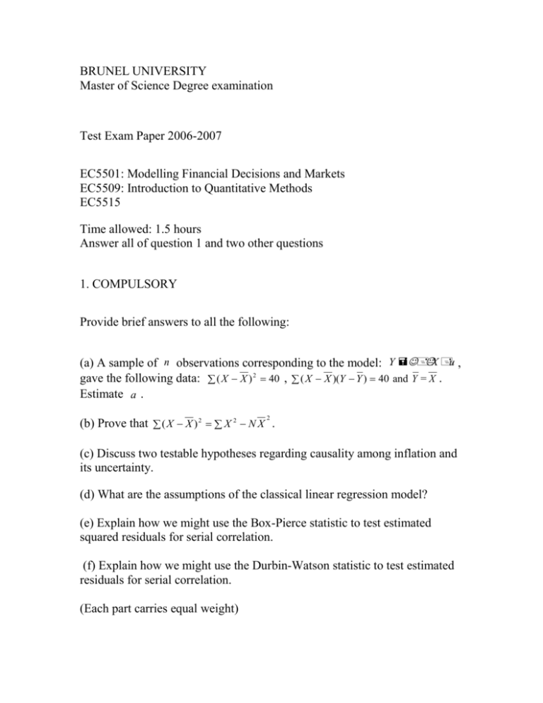
BRUNEL UNIVERSITY
Master of Science Degree examination
Test Exam Paper 2006-2007
EC5501: Modelling Financial Decisions and Markets
EC5509: Introduction to Quantitative Methods
EC5515
Time allowed: 1.5 hours
Answer all of question 1 and two other questions
1. COMPULSORY
Provide brief answers to all the following:
(a) A sample of n observations corresponding to the model: Y X u ,
gave the following data:  ( X  X ) 2  40 ,  ( X  X )(Y  Y )  40 and Y = X .
Estimate a .
2
(b) Prove that  ( X  X ) 2   X 2  N X .
(c) Discuss two testable hypotheses regarding causality among inflation and
its uncertainty.
(d) What are the assumptions of the classical linear regression model?
(e) Explain how we might use the Box-Pierce statistic to test estimated
squared residuals for serial correlation.
(f) Explain how we might use the Durbin-Watson statistic to test estimated
residuals for serial correlation.
(Each part carries equal weight)
ANSWER TWO QUESTIONS FROM THE FOLLOWING:
2. (a) Economic theory supplies the economic interpretation for the predicted
relationships between real (growth) uncertainty and output growth. Discuss
three testable hypotheses regarding causality among these two variables.
(b) An investigator estimates a linear relation for US growth ( yt ):
4
yt    i 1  i yt i  ut , t=1,…,200 . The values of six test statistics are shown
in Table 1. Discuss the results. Is the above equation correctly specified?
(c) Explain how we might use the Box-Pierce statistic to test estimated
residuals for serial correlation.
(Each part carries equal weight)
Y X   u
3. (a) Consider the classical linear regression model
Prove that the least-squares
b

k1

n 1 
n k

k1

n 1.
vector is b X X1 X Y .
(b) The following regression equation is estimated as a production function
for Q :
lnQ 1. 37 
0. 632 lnK 
0. 452 lnL, cov
b k , b l 0. 055,

0.257

0.219
where the standard errors are given in parentheses.
(i)
Test the hypothesis that capital ( K ) and labor ( L ) elasticities of
output are identical.
(ii) Test the hypothesis that there are constant returns to scale.
(Each part carries equal weight)
4. (a) i) Show how various examples of typical hypotheses fit into a general
linear framework: Rb r , where R is a ( q k ) matrix of known constants,
with q k , b is the ( k 1 ) least-squares vector, and r is a q -vector of
known constants.
ii) Show how the least-squares estimator ( b ) of  can be used to test
various hypotheses about  .
(b) The results of least-squares estimation (based on 30 quarterly
observations) of the regression of the actual on predicted interest rates
(three-month U.S. Treasury Bills) were as follows:
r t 0. 24 0. 94 r t e t , RSS 28. 56,

0.86

0.14
where r t is the observed interest rate, and r t is the average expectation of
r t held at the end of the preceding quarter. Figures in parentheses are
estimated standard errors. The sample data on r  give
rt r2 52 .
 rt /30 10 ,
According to the rational expectations hypothesis expectations are unbiased,
that is, the average prediction is equal to the observed realization of the
variable under investigation. Test this claim by reference to announced
predictions and to actual values of the rate of interest on three-month U.S.
Treasury Bills.
(Note: In the above equation all the assumptions of the classical linear
regression model are satisfied; the 5% critical value is F2, 283. 34 ).
(Each part carries equal weight)
5. (a) Explain how we might use White statistic to test for the presence of
heteroscedasticity in the estimated residuals.
(b) A specified equation is Y Xu , with Eu0 and Euu,
where  diag 21 , , 22 . Derive White's correct estimates of the
standard errors of the OLS coefficients.

(c) In the two-variable equation: Yi a bX i , i 1, , n show that var

b2 / 
X X2 .
(Hint: use the fact that the variance-covariance matrix of the ( 2 1 ) leastsquares vector is 2 X X1 )
(Each part carries equal weight)