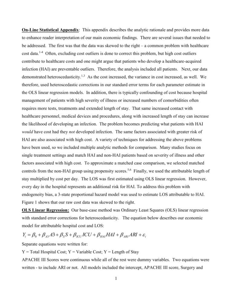
On-Line Statistical Appendix: This appendix describes the analytic rationale and provides more data
to enhance reader interpretation of our main economic findings. There are several issues that needed to
be addressed. The first was that the data was skewed to the right – a common problem with healthcare
cost data.1-4 Often, excluding cost outliers is done to correct this problem, but high cost outliers
contribute to healthcare costs and one might argue that patients who develop a healthcare-acquired
infection (HAI) are preventable outliers. Therefore, the analysis included all patients. Next, our data
demonstrated heteroscedasticity.1,3 As the cost increased, the variance in cost increased, as well. We
therefore, used heteroscedastic corrections in our standard error terms for each parameter estimate in
the OLS linear regression models. In addition, there is typically confounding of cost because hospital
management of patients with high severity of illness or increased numbers of comorbidities often
requires more tests, treatments and extended length of stay. That same increased contact with
healthcare personnel, medical devices and procedures, along with increased length of stay can increase
the likelihood of developing an infection. The problem becomes predicting what patients with HAI
would have cost had they not developed infection. The same factors associated with greater risk of
HAI are also associated with high cost. A variety of techniques for addressing the above problems
have been used, so we included multiple analytic methods for comparison. Many studies focus on
single treatment settings and match HAI and non-HAI patients based on severity of illness and other
factors associated with high cost. To approximate a matched case comparison, we selected matched
controls from the non-HAI group using propensity scores.5,6 Finally, we used the attributable length of
stay multiplied by cost per day. The LOS was first estimated using OLS linear regression. However,
every day in the hospital represents an additional risk for HAI. To address this problem with
endogeneity bias, a 3-state proportional hazard model was used to estimate LOS attributable to HAI.
Figure 1 shows that our raw cost data was skewed to the right.
OLS Linear Regression: Our base-case method was Ordinary Least Squares (OLS) linear regression
with standard error corrections for heteroscedasticity. The equation below describes our economic
model for attributable hospital cost and LOS:
Yi   0   A3 A3   S S   ICU ICU   HAI HAI   ARI ARI   i
Separate equations were written for:
Y = Total Hospital Cost; Y = Variable Cost; Y = Length of Stay
APACHE III Scores were continuous while all of the rest were dummy variables. Two equations were
written - to include ARI or not. All models included the intercept, APACHE III score, Surgery and
1
ICU care. There were two HAI determinations – one where all cases were counted together as “Any
HAI” and a second where each HAI site was individually specified in the economic model. The
classifications for specific infection sites are mutually exclusive; patients with more than one site of
infection were categorized as “Multiple-site”. Single site infections that were not pulmonary,
bloodstream, urinary or surgical site were all categorized as “Other”.
Yi   0   A3 A3   S S   ICU ICU   ARI ARI   PHAI PHAI
  BHAI BHAI  UHAIUHAI   SSI SSI   OHAI OHAI   MSHAI MSHAI   i
Where Y = Total Hospital Cost, Variable Cost or Length of Stay. (See Tables 1 and 2)
Quantile Regression: OLS linear regression estimates the conditional mean based on the values of
the independent variable in the regression equation. For skewed data, “medians” are often preferred
over “means” to describe the central tendency. In similar fashion, Quantile regression using the 0.5 or
“median” quantile to measure the contribution of variables will reduce the contribution of outliers.7,8
Median regression has the same functional form as OLS, but instead of minimizing lest squares,
absolute deviations are minimized. (See Table 3)
n
min
| Y
i 1
i
 ˆ 0  ˆ A3 A3i  ˆS S i  ˆ ICU ICU i  ˆ HAI HAI i  ˆ ARI ARI i |
Winsorizing: Another method of dampening the effects of outliers in skewed data sets, while keeping
them in the analysis is to cap extreme outlier numbers using “Winsorizing”.9,10 As our data was
skewed to the right, all patients were arranged from least to most expensive and the total cost for all
patients in the top 5% were assigned the cost for the next patient just under 5% in the series. Similarly,
for the 98% Winsorizing, the top 2% most expensive patients were all assigned the cost measured for
the next sequential patient. Those costs were:
95% Winsorized
$49,810.74 – This total cost for patient #1,190 out of 1,253 (95%) was applied
to the 63 patients with higher costs.
98% Winsorized
$77,281.67 – This total cost for patient #1,228 of 1,253 (98%) was applied to the
25 patients with higher costs.
After Winsorizing cost, OLS linear regression was performed, as described above with standard errors
assuming a heteroscedastic data distribution. (See Table 3)
2
Semi-log Transformation: Another way to reduce the effect of outliers is to convert the raw
numbers to a logarithm.7 One simple example is to use the Base10 log where: 0 = 0; 10 = 1; 100 = 2,
1,000 = 3, 10,000 = 4; 100,000 = 5. This procedure reduces the relative contributions of very high
numbers in a rightward skewed data distribution. In our methods, we used the natural logarithm. Only
the cost term was log transformed, while all of the predictors such as APACHE III scores remained the
same and the dummy variables remained 1 or 0. When only one half of the equation is logtransformed, it is called “semi-log” transformation. The results are the natural log of the parameter
estimates. The resulting parameter estimate for HAI is then exponentiated. Exp([  HAI ]) – 1 is
interpreted to be the proportional change in cost for HAI over baseline.11 This can be used by facilities
with different financial structures to estimate relative proportional increases in cost due to HAI.
(See Table 3)
ln( Yi )   0   A3 A3   S S   ICU ICU   HAI HAI   ARI ARI   i
Generalized Linear Model: To minimize the effects of skewed data, a generalized linear model
(GLM) with log as link function and gamma distribution, was also performed.1,2,3,12 Rather than
comparing means for cost as done in OLS linear regression procedure, the GLM compares the means
of the natural log of the dependent variable (cost). The gamma distribution of variance was specified.
For retransformation to cost, the parameter estimates are exponentiated in subgroups. To estimate the
cost attributable to HAI, the entire patient sample was organized into 16 subgroups defined by the
presence of Surgery, ICU care, Any ARI or Any HAI. The mean APACHE III was included in the
GLM equation as a cost predictor, but was not used in the retransformation because it would falsely
overestimate HAI cost. It was measured on patient admission, not infection onset. The parameter
estimates for each explanatory variable were exponentiated and multiplied by the variables listed in
each subgroup. The per-patient average predicted cost for each of the 8 subgroups with HAI was
subtracted from the average for the 8 non-HAI subgroups with matching descriptive variables. Each
subgroup average per-patient cost difference was multiplied by the total number of HAIs in that
subgroup. These total differences were summed, and then divided by the total number of HAI (159)
for an overall average HAI cost. We also calculated the average for ARI and non-ARI subgroups
separately.
The disturbance term is assumed to follow a gamma distribution, i.e. εi ~ Г(k, θ), where k is a shape
parameter, and θ is a scale parameter, both positive.
Yi  exp{ 0   S S 2   ICU ICU 2   A3 A3A3   ARI ARI 2   HAI HAI 2   i }
3
Where Surgery, ICU, ARI and HAI are either one or zero and APACHE III score is the mean for the
specific subgroup described by the rest of the equation. (See Tables 4 and 5)
Propensity Scores to Select Matched Controls: Logistic regression was used to determine predictors
of HAI in the sample using APACHE III scores, treatment subgroups (Surgery, ICU), comorbidities,
and ARI. Those comorbidities significantly associated with development of HAI (P < 0.05) were
included in the propensity score used to select matched controls from those who did not develop HAI.
Two propensity scores were developed – one that included concurrent ARI infection and one that did
not. The mean patient cost differences for the two groups – HAI versus matched non-HAI controls
were compared using paired T-tests.5,6 (See Table 6)
Length of Stay Multiplied by Cost per Day: For another measure of the cost attributable to HAI, the
Length of Stay (LOS) attributable to HAI was multiplied by the mean cost per day. Multiple mean
daily cost measures were used – the overall mean for the entire sample, for HAI patients and Non-HAI
patients. Prolonged duration of hospital stay increases patient risk for HAI.13,14,15 That makes it
difficult to determine how many excess days in the hospital are attributable to the HAI alone versus
prolonged LOS acting as a risk factor. Therefore, an alternate LOS was calculated using a multistate
or 3-state proportional hazard model. We used the R package “ChangeLOS” from the Comprehensive
R Archive network (http://www.r-project.org).16 This required finding the date of the first evidence of
HAI for each patient, then calculating a pre-infection and post-infection length of stay. That data was
used in a 3-state proportional hazard model to estimate the LOS attributable to HAI - in distinction
from the pre-infection extended LOS that may have increased patient risk for HAI. One limitation in
our study was that over 25% of patients had multiple HAIs and the 3-state proportional hazard model
only accounted for the start of the first infection.
4
REFERENCES STATISTICAL ABSTRACT
1. Blough DK, Ramsey SD. Using generalized linear models to assess medical care costs.
Health Serv Outcomes Res Methodol 2000; 1(2):185-202.
2. Manning WG, Mullahy J. Estimating log models: to transform or not to transform? J Health
Econ 2001; 20:461-494.
3. Manning WG. The logged dependent variable, heteroscedasticity, and the retransformation
problem. J Health Econ 1998; 17:283-295.
4. Mullahy J. Econometric modeling of health care costs and expenditures: A survey of
analytical issues and related policy considerations. Med Care 2009; 47(7):104-108.
5. Austin PC. A critical appraisal of propensity-score matching in the medical literature
between 1996 and 2003. Stat Med 2008; 27(12):2037-49.
6. Kurth T, Walker AM, Glynn RJ, et al. Results of multivariable logistic regression,
propensity matching, propensity adjustment, and property-based weighing under conditions
of nonuniform effect. Am J Epidemiol 2006; 163:262-270.
7. Kleinbaum DG, Kupper LL, Nizam A, Muller KE. Applied Regression Analysis and Other
Multivariable Methods, 4th edition. Belmont, CA.; Duxbury Press, 2008.
8. Chen CL. An introduction to quantile regression and the QUANTREG procedure. Paper
213-30. SAS Institute Inc. Available at:
www2.SAS.com/proceedings/sugi30/213-30.pdf. (Accessed May 12, 2009).
9. Thomas JW, Ward K. Economic profiling of physician specialists: use of outlier treatment
and episode attribution rules. Inquiry 2006; 43:271-282.
10. Buckley JA, Georgianna TD. Analysis of statistical outliers with application to whole
effluent toxicity testing. Water Environ Res 2001; 73(5):575-583.
11. Krautmann AC, Ciecka J. Interpreting the regression coefficient in semilogarithmic
functions: a note. Indian J of Economics and Business 2006; 5(1):121-125.
12. Diehr P, Yanez D, Ash A, et al. Methods for analyzing health care utilization and costs.
Annu Rev Public Health 1999; 20:125-44.
13. Beyersmann J, Gastmeier P, Grundmann H, et al. Use of multistate models to assess
prolongation of intensive care unit due to nosocomial infection. Infect Control Hosp
Epidemiol 2006; 27(5):493-499.
14. Beyersmann J, Wolkewitz M, and Schumacher M. The impact of time-dependent bias in
proportional hazards modeling. Stat Med 2008; 27(30):6439-6454.
15. Wolkewitz M, Vonberg RP, Grundmann H, et al. Risk factors for the development of
nosocomial pneumonia and mortality on intensive care units: application of competing risks
models. Critical Care 2008; 12(2):R44.
16. Wangler M, Beyersmann J. Package ‘changeLOS’ Version 2.0.9-2. 2008. Available at:
http://cran.r-project.org/web/packages/changeLOS/changeLOS.pdf (Accessed April 19,
2010)
5