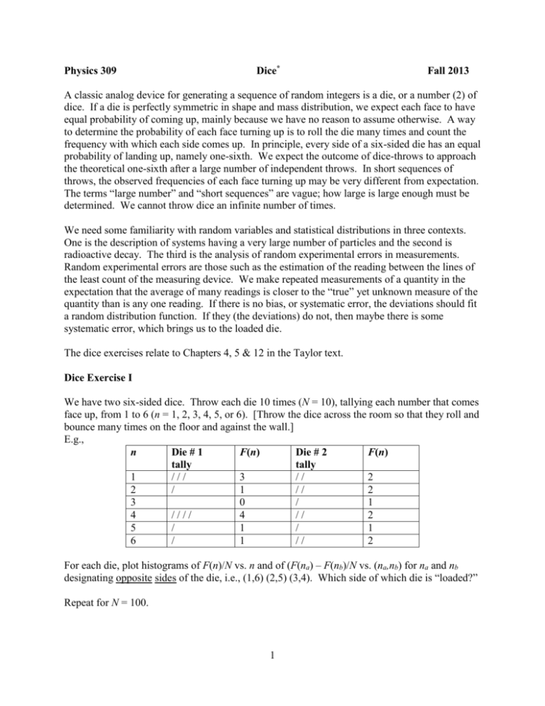
Physics 309
Dice*
Fall 2013
A classic analog device for generating a sequence of random integers is a die, or a number (2) of
dice. If a die is perfectly symmetric in shape and mass distribution, we expect each face to have
equal probability of coming up, mainly because we have no reason to assume otherwise. A way
to determine the probability of each face turning up is to roll the die many times and count the
frequency with which each side comes up. In principle, every side of a six-sided die has an equal
probability of landing up, namely one-sixth. We expect the outcome of dice-throws to approach
the theoretical one-sixth after a large number of independent throws. In short sequences of
throws, the observed frequencies of each face turning up may be very different from expectation.
The terms “large number” and “short sequences” are vague; how large is large enough must be
determined. We cannot throw dice an infinite number of times.
We need some familiarity with random variables and statistical distributions in three contexts.
One is the description of systems having a very large number of particles and the second is
radioactive decay. The third is the analysis of random experimental errors in measurements.
Random experimental errors are those such as the estimation of the reading between the lines of
the least count of the measuring device. We make repeated measurements of a quantity in the
expectation that the average of many readings is closer to the “true” yet unknown measure of the
quantity than is any one reading. If there is no bias, or systematic error, the deviations should fit
a random distribution function. If they (the deviations) do not, then maybe there is some
systematic error, which brings us to the loaded die.
The dice exercises relate to Chapters 4, 5 & 12 in the Taylor text.
Dice Exercise I
We have two six-sided dice. Throw each die 10 times (N = 10), tallying each number that comes
face up, from 1 to 6 (n = 1, 2, 3, 4, 5, or 6). [Throw the dice across the room so that they roll and
bounce many times on the floor and against the wall.]
E.g.,
n
Die # 1
F(n)
Die # 2
F(n)
tally
tally
1
///
3
//
2
2
/
1
//
2
3
0
/
1
4
////
4
//
2
5
/
1
/
1
6
/
1
//
2
For each die, plot histograms of F(n)/N vs. n and of (F(na) – F(nb)/N vs. (na,nb) for na and nb
designating opposite sides of the die, i.e., (1,6) (2,5) (3,4). Which side of which die is “loaded?”
Repeat for N = 100.
1
Now, we investigate the confidence level of our conclusion. We want a quantitative measure of
how sure we are of our designation of the loaded face of the loaded die. One such is the chisquare test. The immediate issue is sample size. Necessarily we toss the dice a finite number of
times. The question is, how well does a finite number of throws replicate the statistics of an
infinite number of throws. The larger the sample size (N) is, the more nearly its frequency
distribution will mimic the frequency distribution of an infinite number of throws, f(n). On the
other hand, if samples of increasing sizes do not approach the statistical behavior of an infinite
sequence of throws, then some form of systematic effect is suspected—the outcomes are not
really random. The chi-square test compares two distributions, or two sample sets. In this case,
we are comparing the frequency distribution of N throws of a die with the ideal random
distribution of N throws of a die.
F ( n )  Nf ( n )2
2  
Nf ( n )
n
2
If   0 , then the observed frequency distribution exactly matches the theoretical distribution,
f(n). But this will never happen; we have to decide how close to matching is “close enough.”
We might be satisfied if the F(n) differed no more from f(n) than one standard deviation of f(n)
for every n. For random events, that would be  Nf ( n ) . If this were the case, then
6
 2  1  6 . The benchmark for the six-sided die, then, is whether  2  6 .
n 1
We’re not done yet. We throw the die a finite number of times, N. It is perfectly possible that
the particular sequence of throws closely matches the theoretically expected frequency
distribution by accident. Another sequence of N throws may very well have a  2  6 . We
must imagine performing a large number of N-sequences of throws, and obtaining a range of  2
 
values which in their turn follow a frequency distribution f  2 . The integral

 f(
2
)d 2  1 .
0
The percentage of the integral for values of  2 that exceed a particular value  o2 is said to be the
confidence level, P, of  o2 . Let’s say that  o2  5 and that P = 25%. This says that if the
outcomes of the throws of the die are random, then there would be a 25% chance that  o2  5 .
The conventional criterion is P = 5%. If we were to obtain a  o2 at a confidence level P < 5%,
we would conclude that the  o2 indicated that the N throws were not in agreement with a random
frequency distribution. I.e., according to the Table below, if  o2  12.6 , then P  5% and we
conclude that the sequence of N rolls of the die are not random—we are 95% sure that the die is
loaded.
Compute the  2 for the N =10 and N = 100 tosses for both die. What do we conclude about the
loading of the two dice?
2
 o2 confidence level for outcomes = 6
Confidence level, P(%)
 o2
99
98
95
90
80
20
10
5
2
1
0.1
0.872
1.134
1.635
2.204
3.070
8.558
10.645
12.592
15.033
16.812
22.457
3
Dice Exercise II
Firstly, we will create a table of random one-digit numbers in the interval [0,9]. We’ll do this by
rolling three 20-sided dice and recording the digit showing on each die. Each 20-sided die has
two of each integer, 0, 1, 2, 3, 4, 5, 6, 7, 8, & 9. (20-sided is icosohedral.) Each digit, then, has
a 2/20 = 1/10 chance of coming up at every toss of a single die. The digits, if the dice are
unbiased, should be uniformly distributed. We will draw numbers from this table throughout this
exercise.
Create a 24x15 table of random digits. Always read the three 20-sided dice in the same order
(red, yellow, blue, for instance).
Limiting distribution
Select a subset of 36 digits from the random number table. Just select the first 36 digits of the
larger table. Record the frequency of occurrence for each digit in [0,9], and make a histogram of
the frequencies. The frequencies of occurrence are the number of times each digit appears
divided by 36. Compute the average and variance of the 36 digits.
Next, select a subset of 120 digits, and a make a frequency histogram, and compute the average
and variance. The frequencies of occurrence are the number of times each digit appears divided
by 120.
Next, make a frequency histogram of all 360 digits, and compute the average and variance.
Comment on the 3 graphs, and sets of averages and variances, particularly in relation to what we
10
expect the frequency distribution, average, and variance to be. n 
 ni
i 1
10
10
, 2 
( n
i 1
i
 n )2
10
Unequal probabilities
Select 100 pairs of digits from the random number table. Take the sum of each pair, producing a
set of 100 numbers in the interval [0,18].
Make a frequency histogram of the numbers [0,18]. Compute the average and variance; compare
with the expected values of the average and variance. To obtain the expected values, we count
the number of ways two numbers in the interval [0,9] can be added to produce a number in
[0,18]. For instance, there are three ways to obtain 16: 7&9, 8&8, and 9&7. The probability of
obtaining 16 in any pair is 3/100 = 3%.
4
Where does the Normal Distribution come in?
Consider the frequency of 7 occurring in the 360-digit random number table. The probability of
a certain number of sevens in a 360-digit random number table is given by the binomial
distribution. The key point here is that the table has a finite number of entries, namely 360.
M!
, with p = 1/10, q=9/10, & M = 360, is the probability of getting n
PN , p ( n )  p n q M n
( M  n )! n!
sevens in 360 throws of one 20-sided die. The normal distribution is the limiting case of the
binomial distribution as M grows very large, but p remains finite, or constant.
( n n )2

1
2
Gn , ( n ) 
e 2 .
 2
By recording the frequencies for all 10 digits in [0,9], in effect we are performing ten 360-throw
repetitions. Use as n and as  2 the expected average frequency of random digits in [0,9] and
10
 ni
10
( n
i
 n )2
M
.
,  2  i 1
10
10
10
The question is, what are the odds of obtaining n sevens in a random sequence of M digits, where
n might be 5, or 40, or 15?
1
1 9
n  Mp  360   36,  2  Mpq  360    32.4 (This is the expected variance.)
10
10 10
If the digits are truly random, then the normal distribution tells the odds that a number of sevens,
n  n , will occur. If we were to obtain an n whose odds of being different from n are not small,
we might come to suspect that the digits were not produced randomly after all. On the other
hand, the normal distribution tells us that obtaining, say, n = 33 sevens in 360 throws of a die is
not really particularly unlikely. At n  n , G(36) = 7%, while G(33) = 6%. What we do, is add
up the probabilities for all n between n  2 and n  2 , and state that there is a 4.6% chance
that we would obtain an n outside that range; i.e., it’s not likely.
How does this relate to measurement? We expect that the average of N independent
measurements will be close to the “true” value of the quantity measured. We do not make an
infinite number of repeated measurements, we make N of them. What are the odds that the
average we obtain from N measurements is within, say, one standard deviation of the “true”
value, as long as there are only random errors in our measurements, as opposed to systematic
errors? It’s 31.7%.
variance, respectively, n 
i 1

 n  n 2


1
2
P 
e 2 dn
 2
Finally, the average or mean of a set of N measurements may be different than the expected
average. Should we repeat sets of N measurements, we would obtain a set of means, of which
we could compute a standard deviation. Turns out that the standard deviation of the mean is
equal to the standard deviation of a set of N measurements divided by N .
 mean 

.
N
Therefore, we would report the measurement as n   mean .
5
Dice Exercise III
There is a 68% chance that the frequency of any digit in [0,9] will be within one standard
deviation of the mean, 95% chance that it will be within two standard deviations. Do the digit
frequencies in the table of 360 random digits meet those criteria?
*
Adapted from Berkeley Physics Laboratory, 2nd ed., Portis and Young, McGraw-Hill, 1971.
6