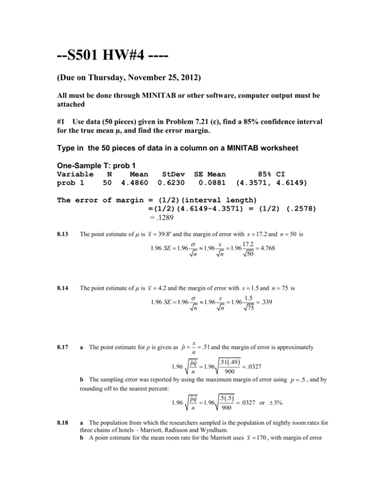
--S501 HW#4 ---(Due on Thursday, November 25, 2012)
All must be done through MINITAB or other software, computer output must be
attached
#1 Use data (50 pieces) given in Problem 7.21 (c), find a 85% confidence interval
for the true mean µ, and find the error margin.
Type in the 50 pieces of data in a column on a MINITAB worksheet
One-Sample T: prob 1
Variable
N
Mean
prob 1
50 4.4860
StDev
0.6230
SE Mean
0.0881
85% CI
(4.3571, 4.6149)
The error of margin = (1/2)(interval length)
=(1/2)(4.6149-4.3571) = (1/2) (.2578)
= .1289
8.13
The point estimate of  is x  39.8o and the margin of error with s  17.2 and n  50 is
1.96 SE  1.96
8.14
n
 1.96
s
n
 1.96
17.2
50
 4.768
The point estimate of  is x  4.2 and the margin of error with s  1.5 and n  75 is
1.96 SE  1.96
8.17

a The point estimate for p is given as pˆ 

n
 1.96
s
n
 1.96
1.5
75
 .339
x
 .51 and the margin of error is approximately
n
.51.49 
ˆˆ
pq
 1.96
 .0327
n
900
b The sampling error was reported by using the maximum margin of error using p  .5 , and by
rounding off to the nearest percent:
1.96
1.96
8.18
.5 .5 
ˆˆ
pq
 1.96
 .0327 or  3%
n
900
a The population from which the researchers sampled is the population of nightly room rates for
three chains of hotels – Marriott, Radisson and Wyndham.
b A point estimate for the mean room rate for the Marriott uses x  170 , with margin of error
1.96 SE  1.96

 1.96
s
 1.96
17.5
 4.85
n
n
50
c A point estimate for the mean room rate for the Radisson uses x  145 , with margin of error

s
10
1.96 SE  1.96
 1.96
 1.96
 2.77
n
n
50
d A point estimate for the mean room rate for the Wyndham uses x  150 , with margin of error

s
16.5
1.96 SE  1.96
 1.96
 1.96
 4.57
n
n
50
e The graphical comparison of parts b, c and d is shown below. The Radisson seems to have
lower and less variable rates than the other two hotels.
200
Avg Room Rate
150
100
50
0
Marriott
Radisson
Wyndham
Hotel
8.30
With n  30, x  145 and s  .0051 , a 90% confidence interval for  is approximated by
x  1.645
s
n
 .145  1.645
.0051
30
 .145  .0015 or .1435    .1465
One-Sample T
N
30
8.31
Mean
0.145000
StDev
0.005100
SE Mean
0.000931
90% CI
(0.143418, 0.146582)
With n  40, x  3.7 and s  .5 and   .01 , a 99% confidence interval for  is approximated by
x  2.58
s
n
 3.7  2.58
.5
40
 3.7  .204 or 3.496    3.904
In repeated sampling, 99% of all intervals constructed in this manner will enclose  . Hence, we
are fairly certain that this particular interval contains  . (In order for this to be true, the sample
must be randomly selected.)
One-Sample T
N
Mean
StDev
40 3.7000 0.5000
SE Mean
0.0791
99% CI
(3.4859, 3.9141)
We assumed that the PH values follow a normal
distribution in order that the confidence interval is valid.
8.32
a An approximate 95% confidence interval for p is
pˆ  1.96
or
.54 .46 
ˆˆ
pq
 .54  1.96
 .54  .049
n
400
.491  p  .589 .
Test and CI for One Proportion
Sample
X
N Sample p
1
216 400 0.540000
95% CI
(0.489766, 0.589638)
b An approximate 95% confidence interval for p is
.30 .70 
ˆˆ
pq
pˆ  1.96
 .30  1.96
 .30  .048
n
350
or .252  p  .348 .
Test and CI for One Proportion
Sample
X
N Sample p
1
105 350 0.300000
8.34
95% CI
(0.252434, 0.350988)
a The 90% confidence interval for p is
pˆ  1.645
or
.39 .61
ˆˆ
pq
 .39  1.645
 .39  .025
n
1002
.365  p  .415 .
Test and CI for One Proportion
Sample
X
N Sample p
1
391 1002 0.390220
90% CI
(0.364637, 0.416282)
b The 90% confidence interval for p is
pˆ  1.645
.53 .47 
ˆˆ
pq
 .53  1.645
 .53  .026
n
1002
or .504  p  .556 .
Test and CI for One Proportion
Sample
1
8.45
X
531
N
1002
Sample p
0.529940
90% CI
(0.503466, 0.556284)
a The point estimate of the difference 1  2 is
x1  x2  53,659  51,042  2617
and the margin of error is
1.96
 12
n1

 22
n2
1.96
22252 23752

 902.08
50
50
b Since the estimate of the difference 1  2 is 2617  902.08  1714.92 which is greater than
the margin error ─ it seems that there is a significant difference in starting salaries, it is likely that
the mean for chemical engineering majors is larger than the mean for computer science majors.
8.48
a The 99% confidence interval for 1  2 is approximately
 x1  x2   2.58
s12 s22

n1 n2
42 10 2

30 40
 8  4.49 or  12.49   1   2   3.51
15  23  2.58
Two-Sample T-Test and CI
Sample
N
Mean StDev SE Mean
1
30 15.00
4.00
0.73
2
40
23.0
10.0
1.6
Difference = mu (1) - mu (2)
Estimate for difference: -8.00
99% CI for difference: (-12.65, -3.35)
b Since the confidence interval in part a has two negative endpoints, it does not contain the value
1  2  0 . Hence, it is not likely that the means are equal. It appears that there is a real
difference in the mean times to completion for the two groups.
8.57
a With pˆ1 
x1
x
 .62 and pˆ 2  2  .35 . The approximate 99% confidence interval is
96
105
 pˆ1  pˆ 2   2.58
pˆ1qˆ1 pˆ 2 qˆ2

n1
n2
.62 .38  .35 .65 

96
105
.27  .175 or .095   p1  p2   .445
.62  .35   2.58
Test and CI for Two Proportions
Sample
X
N Sample p
1
60
96 0.625000
2
37 105 0.352381
Difference = p (1) - p (2)
Estimate for difference: 0.272619
99% CI for difference: (0.0976366, 0.447602)
8.59
b
Since the value p1  p2  0 is not in the confidence interval, it is not likely that p1  p2 . You
should conclude that there is a difference in the proportion of people with colds for the two groups.
c
The data shows the opposite effect from what you might expect. It appears that coming into
contact with more people actually decreases the probability of getting a cold. Perhaps the more
you are out among a variety of people, the more immune your system becomes to cold germs and
viruses.
Calculate pˆ1 
x1 120
x
54

 .7 and pˆ 2  2 
 .54 . The approximate 90% confidence interval
n1 180
n2 100
is
 pˆ1  pˆ 2   1.645
pˆ1qˆ1 pˆ 2 qˆ2

n1
n2
.7 .3 .54 .46 

180
100
.16  .099 or .061   p1  p2   .259
.7  .54   1.645
Test and CI for Two Proportions
Sample
X
N Sample p
1
126 180 0.700000
2
54 100 0.540000
Difference = p (1) - p (2)
Estimate for difference: 0.16
90% CI for difference: (0.0606167, 0.259383)
Intervals constructed in this manner will enclose the true value of p1  p2 90% of the time in repeated
sampling. Hence, we are fairly certain that this particular interval encloses p1  p2 . Since the
interval does not include zero, it is likely that the percentage of first born for graduates is
significantly higher than that of nongraduates.
8.68
It is necessary to find the sample size required to estimate a certain parameter to within a given
bound with confidence 1    . Recall from Section 8.5 that we may estimate a parameter with
1    confidence within the interval (estimator)
 z 2  (std error of estimator). Thus, z 2  (std
error of estimator) provides the margin of error with 1    confidence. The experimenter will
specify a given bound B. If we let z 2  (std error of estimator)  B , we will be 1    confident
that the estimator will lie within B units of the parameter of interest.
For this exercise, the parameter of interest is  , B  1.6 and 1    .95 . Hence, we must have
1.96

n
 1.6  1.96
n
1.96 12.7 
12.7
n
 1.6
 15.5575
1.6
n  242.04 or n  243
8.69
pq
. Assuming
n
maximum variation, which occurs if p  .3 (since we suspect that .1  p  .3 ) and z.025  1.96 , we
have
For this exercise, B  .04 for the binomial estimator p̂ , where SE  pˆ  
1.96 pˆ  B  1.96
.3 .7 
1.96
8.70
n
n
1.96 .3 .7 
.04
 n  504.21 or n  505
In this exercise, the parameter of interest is 1  2 , n1  n2  n , and  12   22  27.8 . Then we
must have
z 2  (std error of x1  x2 )  B
1.645
n
8.71
 .04 
pq
B
n
 12
n1

 22
n2
 .17  1.645
27.8 27.8

 .17
n
n
1.645 55.6
 n  5206.06 or n1  n2  5207
.17
In this exercise, the parameter of interest is p1  p2 , n1  n2  n , and B  .05 . Since we have no
prior knowledge about p1 and p2 , we assume the largest possible variation, which occurs if
p1  p2  .5 . Then
z 2  (std error of pˆ1  pˆ 2 )  B
z.01
p1q1 p2 q2

 .05  2.33
n1
n2
n
8.91
.5.5 .5.5
n

n
 .05
2.33 .5
 n  1085.78 or n1  n2  1086
.05
a Define sample #1 as the sample of 482 women and sample #2 as the sample of 356 men. Then
pˆ1  .5 and pˆ 2  .75 .
b The approximate 95% confidence interval is
pˆ qˆ
pˆ qˆ
 pˆ1  pˆ 2   1.96 1 1  2 2
n1
n2
.5 .5  .75 .25 

482
356
 .25  .063 or  .313   p1  p2   .187
.5  .75  1.96
c
Since the value p1  p2  0 is not in the confidence interval, it is unlikely that p1  p2 . Since
all the probable values of p1  p2 are negative, the proportion of men of Wall Street who have
children appears to be larger than the proportion of women.
8.92 The best sample estimator for the mean  is x   xi n . Therefore, the estimated value of  is
x  9.7 .
One-Sample T
N
Mean StDev
35 9.700 5.800
SE Mean
0.980
95% CI
(7.708, 11.692)
The margin of error is E= (1/2)(11.692-7.708)= 1.992
(the computer used a better approximation rather than plain CLT)
or

s
 5.8 
1.96 x  1.96
 1.96
 1.96 
  1.92
n
n
 35 
The population in this exercise is the difference in blood pressure for all collegeaged smokers between the beginning of the experiment and five years later.
8.102
Using the range approximation to obtain an estimate of  , we have
R 13, 000  4800
 
 2050
4
4
and the desired value of n is obtained:

2050
1.96
 B  1.96
 500  n  64.58 or n  65
n
n
8.103
It is assumed that p  .2 and that the desired bound is .01. Hence,
1.96
8.107
1.96 .05 .95 
pq
 .01 
n
 42.72
n
.01
n  1824.76 or n  1825
a The approximate 95% confidence interval for  is
x  1.96
or 2.837    3.087 .
s
n
 2.962  1.96
.529
69
 2.962  .125
One-Sample T
N
69
Mean
2.9620
StDev
0.5290
SE Mean
0.0637
95% CI
(2.8349, 3.0891)
b In order to cut the interval in half, the sample size must increase by 4. If this is done, the new
half-width of the confidence interval is

1
 
1.96
 1.96
.
2
4n
n

Hence, in this case, the new sample size is 4  69   276 .
7.75
Type in the 25 defective numbers on column, say, Defectives
Use calculator to compute Def-Rate = Defectives / 100
a
Construction of a p chart based on data. The average proportion of defectives is
.04  .02   .03
p
 .032
25
and the control limits are
UCL  p  3
p (1  p )
.032(.968)
 .032  3
 .0848
n
100
p (1  p )
.032(.968)
 .032  3
 .0208
n
100
If subsequent samples do not stay within the limits, UCL  .0848 and LCL  0 , the process
should be checked.
LCL  p  3
and
Problem #7.75 Defective Rate Control Chart (n=100)
0.10
UCL=0.0863
Individual Value
0.08
0.06
0.04
_
X=0.032
0.02
0.00
-0.02
LCL=-0.0223
1
3
5
7
9
11 13 15
Observation
17
19
21
23
25
b From part a, we must have pˆ  .0848 .
c An erroneous conclusion will have occurred if in fact p  .0848 and the sample
has produced pˆ  .15 by chance. One can obtain an upper bound on the
probability of this particular type of error by calculating P  pˆ  .15 when p  .0848 .
7.78
( Plot 30 observed data against a specified control chart)
a If the process is in control, the mean weight per can is 21 ounces, and the
standard deviation is 1.2 ounces. .
With n  5 , the upper and lower control limits are
21 ± 3 ( 1.2 / SQRT(5) ) = 21 ± 3 (.5366) = 21 ± 1.61
or CLC= 21 – 1.61 = 19.39, and UCL= 21 + 1.61 = 22.61
b
.
Using specification. Mean =21, SE of Average weight of 5 cans = 1.2 / SQRT(5) = 0.5366
Stat  Control Charts  Variable for individuals  Individuals
Fill in Variable Name, Click ‘I Chart Options’ , fill in Mean =21, and Standard
deviation = .5366, OK, OK
Problem #7.78 Average Weight Control Chart Using Specification
1
23
1
Individual Value
UCL=22.610
22
_
X=21
21
20
LCL=19.390
19
1
4
7
10
13
16
19
Observation
22
25
28
Two samples exceed the bounds (#1, #18); the process is probably out of control at these two time points.
Descriptive Statistics: AvgWeight
Variable N
Mean SE-Mean StDev
AvgWeight 30 21.20 0.144 0.788
Variable
AvgWeight
Min
Q1
Q2
Q3
19.9 20.55 21.30 21.600
Maximum
23.100
The average weight for the 30 samples is 21.2 ounces which
is a little bit higher than the specification. The StDev
(the standard deviation of the average of 5 cans) is 0.788
which is also higher than the specification of 0.5366
ounces.