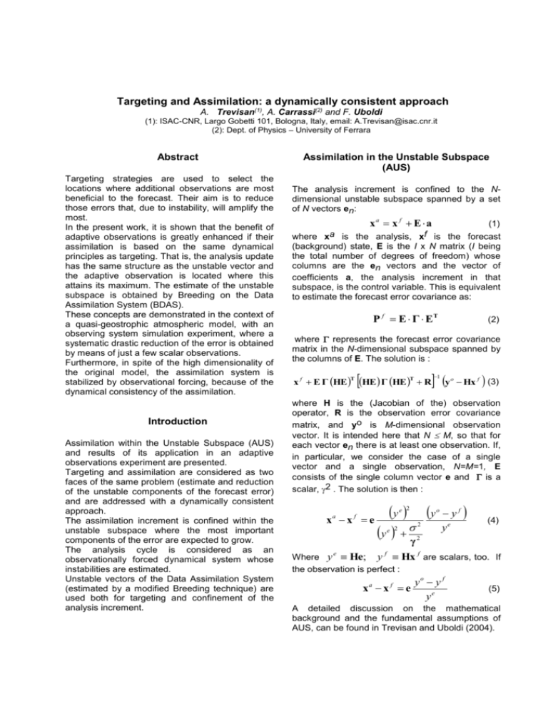
Targeting and Assimilation: a dynamically consistent approach
A. Trevisan(1), A. Carrassi(2) and F. Uboldi
(1): ISAC-CNR, Largo Gobetti 101, Bologna, Italy, email: A.Trevisan@isac.cnr.it
(2): Dept. of Physics – University of Ferrara
Abstract
Targeting strategies are used to select the
locations where additional observations are most
beneficial to the forecast. Their aim is to reduce
those errors that, due to instability, will amplify the
most.
In the present work, it is shown that the benefit of
adaptive observations is greatly enhanced if their
assimilation is based on the same dynamical
principles as targeting. That is, the analysis update
has the same structure as the unstable vector and
the adaptive observation is located where this
attains its maximum. The estimate of the unstable
subspace is obtained by Breeding on the Data
Assimilation System (BDAS).
These concepts are demonstrated in the context of
a quasi-geostrophic atmospheric model, with an
observing system simulation experiment, where a
systematic drastic reduction of the error is obtained
by means of just a few scalar observations.
Furthermore, in spite of the high dimensionality of
the original model, the assimilation system is
stabilized by observational forcing, because of the
dynamical consistency of the assimilation.
Introduction
Assimilation within the Unstable Subspace (AUS)
and results of its application in an adaptive
observations experiment are presented.
Targeting and assimilation are considered as two
faces of the same problem (estimate and reduction
of the unstable components of the forecast error)
and are addressed with a dynamically consistent
approach.
The assimilation increment is confined within the
unstable subspace where the most important
components of the error are expected to grow.
The analysis cycle is considered as an
observationally forced dynamical system whose
instabilities are estimated.
Unstable vectors of the Data Assimilation System
(estimated by a modified Breeding technique) are
used both for targeting and confinement of the
analysis increment.
Assimilation in the Unstable Subspace
(AUS)
The analysis increment is confined to the Ndimensional unstable subspace spanned by a set
of N vectors en:
xa  x f  E  a
(1)
a
f
where x is the analysis, x is the forecast
(background) state, E is the I x N matrix (I being
the total number of degrees of freedom) whose
columns are the en vectors and the vector of
coefficients a, the analysis increment in that
subspace, is the control variable. This is equivalent
to estimate the forecast error covariance as:
P f  E  Γ  ET
(2)
where  represents the forecast error covariance
matrix in the N-dimensional subspace spanned by
the columns of E. The solution is :
x f  E Γ HE 
T
HE Γ HE
T
R
 y
1
o

 Hx f (3)
where H is the (Jacobian of the) observation
operator, R is the observation error covariance
matrix, and yo is M-dimensional observation
vector. It is intended here that N  M, so that for
each vector en there is at least one observation. If,
in particular, we consider the case of a single
vector and a single observation, N=M=1, E
consists of the single column vector e and  is a
scalar, 2 . The solution is then :
x x
a
y  y
e
y   γ
e 2
f
e 2
2
o
 yf
ye

(4)
2
Where y  He; y  Hx are scalars, too. If
the observation is perfect :
e
f
xa  x f  e
f
yo  y f
ye
(5)
A detailed discussion on the mathematical
background and the fundamental assumptions of
AUS, can be found in Trevisan and Uboldi (2004).
Estimate of the unstable subspace
The estimate of the unstable vectors, columns of
E, are estimated by a modified form of breeding
(Toth and Kalnay, 1997). Since our aim is to
estimate the instabilities of the complete analysisforecast cycle solution, we let the perturbed
trajectories undergo the same observational
forcing as the control trajectory. What is called
breeding on the data assimilation system (BDAS)
is similar to the standard breeding technique, the
main difference being the application of the
analysis step to the perturbed trajectories (Carrassi
et al. 2005).
Experiments
In the following, the main steps for the
implementation of AUS in targeting and
assimilation experiments are summarized:





Estimate of the unstable subspace is
obtained by BDAS;
Targeted observations are placed at
locations where bred vectors en have
maximum component;
A wide (2500km) Gaussian modulating
function is used to isolate the regional
structure of the bred vectors;
A small number N of Bred Vectors are
used to construct the matrix E;
Use E in (3) to perform the analysis;
Experiments are performed using a quasigeostrophic periodic channel model (Rotunno and
Bao, 1996) with 64-longitudinal and 32-latitudinal
grid points and 5 vertical levels where potential
vorticity is specified. The perfect model assumption
is made. A fixed observational network, consisting
of vertical sounding, completely covers the
western-most third of the domain (land,
longitudinal grid points 1-20). All land observations
are assimilated by means of a 3DVAR algorithm
(Morss et al., 1999). The rest of the domain
(ocean) is completely void of observations except
for a single observation adaptively located at each
analysis step. We compare results of two different
sets of experiments:

Experiment type I: all observations, fixed
and adaptive, are assimilated by means of
3DVAR

Experiment type II: the fixed observations
are assimilated by means of 3DVAR; the
adaptive observations by means of AUS
In experiments type I the adaptive observation
consists of a complete vertical sounding measuring
temperature
and
the
horizontal
velocity
components. On the other hand, in experiments
type II the adaptive observation consists of a single
temperature observation. We point out that in both
sets of experiments the adaptive observation is
placed where the current bred vector attains its
maximum amplitude.
In all experiments a single bred vector is used at
each analysis step. The breeding time has been
set to 10 days after optimization (Carrassi, 2005).
After being used for targeting (and assimilation in
experiments type II) the bred vector is discarded
and a new perturbation is introduced.
Results
All results presented here are obtained
years long simulated assimilation
Experiments are performed using both
(labeled by P) and noisy (labeled
observations.
with 2
cycles.
perfect
by N)
- Perfect Observations
Fig. 1 shows the normalized (with respect to
natural variability) RMS analysis error as a function
of time. The dotted line refers to exp. I-P (where
the adaptive vertical sounding is assimilated by
3DVAR) while the continuous one refers to exp. IIP that uses (5) to assimilate the adaptive
temperature observation over the ocean.
FIG (1): Normalized RMS analysis error as a function of
time. The error is expressed in potential enstrophy norm
and it is normalized by natural variability. Dotted line: I-P;
Continuous Line: II-P
After about 60 days the average analysis error of
exp. II-P (continuous line) drops below 10% of
natural variability and it never exceeds it
afterwards. The improvement with respect to the
3DVAR experiment is evident. Table 1 contains the
space and time average error from the following
experiments: an experiment with only fixed land
observations assimilated by 3DVAR (Land-Obs),
an experiment where the location of the adaptive
vertical sounding is randomly chosen (RandomObs) and experiments I-P and II-P.
Experiment
RMS
Analysis
Error
Land-Obs
Random-Obs
I-P
II-P
0.43
0.38
0.35
0.02
TABLE 1: Space and time (after 150 days transient)
average analysis error, normalized by natural variability,
for the indicated experiments.
As could be anticipated, the introduction of the
randomly located observation, over the large data
void area, leads to an improvement that is however
more significant when it is located using BDAS (IP). This proves that BDAS is efficient in capturing
the real system instabilities. Finally the largest
improvement is obtained when the ocean
observation is located by BDAS and assimilated by
AUS (II-P).
dimension 21). This demonstrates that, with
respect to 3DVAR, AUS better exploits a smaller
amount of information.
The upper and middle panels of fig. 2 show the
normalized time and vertical average RMS
analysis error for experiments I-P and II-P
respectively. In both cases an initial transient of
150 days has been omitted when calculating the
mean. The analysis error domain distribution
reflects the particular observational network: larger
error values are found in the data void region
(longitudinal grid points 21-64) and an eastward
error advection influences the land area. Anyhow,
apart from these common features, the most
relevant difference between I-P and II-P is the
order of magnitude of errors; as already evident
from fig. 1 in I-P the error is strongly reduced with
respect to II-P. The curves in the lower panel
represent the RMS analysis error as a function of
longitude. We see that the error over the ocean
using AUS (II-P) is everywhere smaller than the
minimum error (over land) using 3DVAR (I-P).
- Stability Analysis
Data assimilation systems constrain the control
trajectory to remain ‘close’ to the true trajectory.
The assimilation of observations itself can be
naturally seen as a forcing on the model dynamics.
Therefore the analysis cycle can be considered as
an observationally forced dynamical system whose
stability can be studied.
The QG model at the present resolution (i.e. the
system without the observational forcing)
possesses 25 positive Lyapunov exponents. The
leading exponent is equal to 0.32 day-1 that implies
a doubling time of about 2 days and the KaplanYorke dimension is approximately 69.07. Fig. 3
shows the leading exponent for the data
assimilation systems of experiments I-P and II-P.
The values are obtained averaging over all
previous instants. After about 100 days the
exponent relative to II-P reaches negative values
and it remains negative afterwards.
FIG (2): Upper panel: Normalized time and vertical
average RMS analysis error from experiment I-P. Middle
panel: Normalized time and vertical average RMS
analysis error from experiment II-P. Lower panel:
Normalized time vertical and latitudinal average RMS
analysis error; continuous line: I-P; dotted line: II-P.
It should be reminded here that in II-P the adaptive
observation is a single temperature observation (y0
is a scalar) while in all other cases, including II-P it
consists of a complete vertical sounding (y0 has
FIG (3): Leading Lyapunov exponent of the assimilation
systems as a function of time. Dotted line: I-P (3DVar);
Continuous Line: II-P (AUS). Values are averaged over
all previous instants. The growth rate is expressed in
units of days-1.
A negative leading Lyapunov exponent indicates
that the observational forcing stabilizes the
solution. On the other hand the forcing by 3DVAR
reduces the leading growth rate of the free system
but is unable to stabilize the solution.
Fig. 5 is the same as fig. 2 (bottom panel). It shows
the normalized latitudinal, vertical and time
average RMS analysis error for I-N and II-N.
- Noisy Observations
Assessment of the value of adaptive observations
from field campaign is still underway and the
results so far are controversial. The main
conclusion of this work is that the benefit of
adaptive observations is greatly enhanced if their
assimilation is based on the same dynamical
principles as targeting. Results show that a few
carefully selected and properly assimilated
observations are sufficient to control the
instabilities of the Data Assimilation System and
obtain a drastic reduction of the analysis error.
Further results (Uboldi et al., 2005) obtained in the
context of a primitive equation ocean model and
regular observational network are also very
encouraging. The extension to the four
dimensional case is in progress. The success
obtained so far makes us confident that, even in an
operational environment with real observations,
this method can yield significant improvement of
the assimilation performance.
Although the perfect observations case represents
an important idealized simplification and allows a
first assimilation performance comparison, noisy
observations experiments better represent real
conditions. Therefore a comparison is made also in
this context.
We use the same observational configuration of IP and II-P but reduce the assimilation interval from
12 to 6 hr. The assimilation of the isolated ocean
observation in II-N is made by applying (4). In this
case therefore we need to estimate the coefficient
 representing the background error projection on
the unstable direction e. In the simple case of a
single unstable vector at each analysis time,  is a
scalar coefficient that can be easily estimated on a
statistical basis (Carrassi et al., 2005).
Fig. 4 is the same as fig. 1 but using noisy
observations. Although less spectacular than in the
prefect observations case, a drastic reduction of
the analysis error is obtained using AUS.
Conclusions
References
Carrassi A., 2005. Geophysical Data Analysis: A new
dynamically based assimilation method. PhD thesis,
University
of
Ferrara,
Italy,
120
pp.
(www.isac.cnr.it/~dinamica/predictability/)
Carrassi A., A. Trevisan and F. Uboldi, 2005.
Deterministic Data Assimilation and Targeting by
Breeding on the Data Assimilation System. In review for
J. Atmos. Sci..
FIG (4): Same as fig (1); Dotted line: Experiment I-N;
Continuous Line: Experiment II-N
Morss R., 1999. Adaptive Observations: Idealized
sampling strategy for improving numerical weather
prediction. PhD thesis, Massachussets of Technology,
Cambridge, MA, 225 pp.
Rotunno R., and J. W. Bao, 1996. A case study of
cyclogenesis using a model hierarchy. Mon. Wea. Rev.,
124, 1051-1066
Trevisan A., and F. Uboldi, 2004. Assimilation of
standard and targeted observation within the unstable
subspace of the observation-analysis-forecast cycle
system. J. Atmos. Sci., 61, 103-113
Uboldi F., A. Trevisan and A. Carrassi, 2005. Developing
a Dynamically Based Assimilation Method for Targeted
and Standard Observations. Nonl. Pr. Geo., 12, 149-156
FIG (5): Same as fig (2c); Dotted line: Experiment I-N;
Continuous Line: Experiment II-N