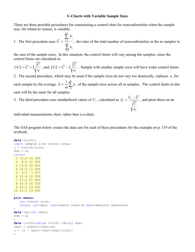
U-Charts with Variable Sample Sizes
There are three possible procedures for constructing a control chart for nonconformities when the sample
size, for whatever reason, is variable.
m
1. The first procedure uses U 
X
i 1
m
n
i 1
i
, the ratio of the total number of nonconformities in the m samples to
i
the sum of the sample sizes. In this situation, the control limits will vary among the samples, since the
control limits are calculated as
UCL  U  3
U
U
, and LCL  U  3
. Sample with smaller sample sizes will have wider control limits.
ni
ni
2. The second procedure, which may be used if the sample sizes do not vary too drastically, replaces ni for
1 m
 ni of the sample sizes across all m samples. The control limits in this
m i 1
case will be the same for all samples.
U U
3. The third procedure uses standardized values of U i , calculated as Z i  i
, and plots these on an
U
ni
individual measurements chart, rather than a u-chart.
each sample by the average, n 
The SAS program below creates the data sets for each of these procedures for the example on p. 319 of the
textbook.
data cloth1;
input sample size noncon area;
u = noncon/size;
dum = 1;
cards;
1 10.0 14 500
2 8.0 12 400
3 13.0 20 650
4 10.0 11 500
5 9.5 7 475
6 10.0 10 500
7 12.0 21 600
8 10.5 16 525
9 12.0 19 600
10 12.5 23 625
;
proc means;
var noncon size;
output out=desc sum=sumnon sumsize mean=meannon meansize;
;
data two;set desc;
dum = 1;
;
data cloth2;merge cloth1 two;by dum;
ubar = sumnon/sumsize;
z = (u - ubar)/sqrt(ubar/size);
;
proc print;
;
run;
1. To create the u-chart according to procedure 1, we run the program, then:
a) Choose Solutions, Analysis, Quality Improvement, Control Charts.
b) For Active Data Set, choose “Cloth1.” For Type of Chart, choose “u-chart.” Then enter the
variable “size” as the Sample Size. For Process Variable, choose “noncon,” the number of
nonconformities in a sample. For Subgroup Variable, choose “sample.” For Method for Obtaining
Limits, choose “compute from the data.”
c) Click Run.
2. To create the chart according to procedure 2, we run the program, then:
a) Record the values of U (in this case 1.4236) and n (in this case 15.3) obtained from SAS PROC\
MEANS. These values will be used to calculate the control limits.
b) Follow the same procedure as in step (b) above, but for Sample Size, enter 15.3, and for Method
for Obtaining Limits, choose “enter the limits to be used.” These limits are
UCL  U  3
U
1.4236
 1.4236  3
 2.3387 , and
n
15.3
U
1.4236
 1.4236  3
 0.5085
n
15.3
c) Click Run.
3. To create the individual measurements chart using the standardized values of U, run the program, then:
a) For Active Data Set, choose “Cloth2.” For Type of Chart, choose “Individual measurements and
moving range.” For Process Variable, choose “z.” For Subgroup Variable, choose “sample.” For
Methods for Obtaining Limits, choose “Enter standard values to be used in computations.” The
process mean will be 0 and the standard deviation will be 1.
b) Click Run.
LCL  U  3