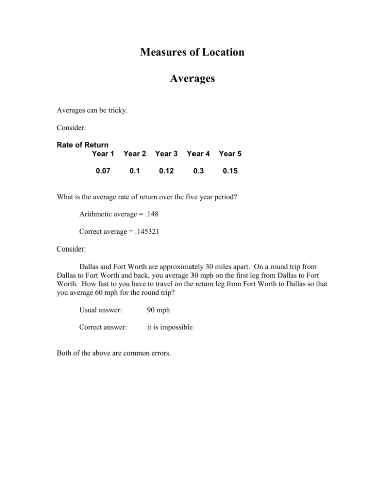
Measures of Location
Averages
Averages can be tricky.
Consider:
Rate of Return
Year 1
Year 2
Year 3
Year 4
Year 5
0.1
0.12
0.3
0.15
0.07
What is the average rate of return over the five year period?
Arithmetic average = .148
Correct average = .145321
Consider:
Dallas and Fort Worth are approximately 30 miles apart. On a round trip from
Dallas to Fort Worth and back, you average 30 mph on the first leg from Dallas to Fort
Worth. How fast to you have to travel on the return leg from Fort Worth to Dallas so that
you average 60 mph for the round trip?
Usual answer:
90 mph
Correct answer:
it is impossible
Both of the above are common errors.
Measures of Location
The Arithmetic Average
The arithmetic average of a set of values is the sum of the values divided by the
number of values.
If x1, x2, . . . . xn represent the n numerical values from a random sample, then the
formula for the sample mean is:
x   xi n
i
To find the average( when I use this term subsequently, I will mean the
arithmetic average), using EXCEL, one uses the function “average”. It is used just like
the “median” function.
Specifically, one types =average( range of data). For the data on steel thickness,
you would have something that looks like the below:
By closing the parentheses, you get the average for the data as 354.55.
Computation of the Arithmetic Mean
From Grouped Data
If we do not have the raw data but only the frequency distribution of the data , the
formula for the sample mean becomes:
x
i
f m /n
i
i
EXCEL does not compute this formula directly. To compute this in EXCEL for
the steel thickness data, one can use the following procedure:
Interval
341.5
344.5
347.5
350.5
353.5
356.5
359.5
362.5
344.5
347.5
350.5
353.5
356.5
359.5
362.5
365.5
m(i)
Midpoint
f(i)
Freq
f(i)*m(i)
343
346
349
352
355
358
361
364
1
3
8
8
20
13
5
2
343
1038
2792
2816
7100
4654
1805
728
60
21276
Average
354.6
If one defines the proportion of observations in a bin as
pf
i
i
/n
then the formula for the mean from grouped data (and also the formula for a discrete
probability distribution) is:
x   pi mi
i
Using the above, it is then possible to generalize the definition of the mean for
data from a continuous distribution with probability density function f(x) as:


 xf ( x)dx

Computation with the Average
Consider the problem of having two groups of people, 50 people in Group 1 with
an average hourly wage of $15.00 and 100 people in Group 2 with an average hourly
wage of $17.00, can I find the mean of the pooled group of 150 people.
The average of the pooled group is just the total hourly wages of all 150 people
divided by the 150 people. Using the formula for the arithmetic average, one can show
that:
nx   xi
i
Therefore the sum of the hourly wages in the first group is 50 x 15 = 750.
The sum of the hour wages in the second group is 100 x 17 = 1700. Finally the mean of
the pooled group is:
pooled average = (750 + 1700)/(50 + 100) = $16.33
This can be written in formula terms as:
x
pooled
 (n1 x1  n2 x2) / (n1  n2)
This is a special case of the formula for multiple groups:
x
pooled
  ni xi /  ni
i
i
Consider the following example which we discussed previously in connection
with the median:
Average
Group
1
Group
2
Change
5
10
15
20
25
4
12
18
19
23
-1
2
3
-1
-2
15
15.2
0.2
Notice that the change in the means is the same as the mean of the changes.
Summary
Criterion
Median
Mean
Ease of Understanding
High
Reasonable
Computation
Moderate
Easy
Effect of Outliers
None
High
Use in Further Computation
None
Easy
Accuracy for Inference to
Population for fixed sample
of size n
25% worse than mean
Baseline
Simpson’s Paradox
Consider the following data found in the file “meandemo.xls:
Males
Male
Average
Prof
35
60,000
5
65,000
Assoc Prof
25
50,000
20
55,000
Asst Prof
15
40,000
15
45,000
Average
Female
Females Average
52,667
52,500
Or the following data also found in the file “meandemo.xls”:
Time 1
Group 1
30
35
48
Group 2
14
85
98
Group 3
60
63
65
All
Groups
Time 1
Median
Time 2
Time 2
Median
Median
Change
35
31
32
75
32
-3
85
60
83
85
83
-2
63
61
62
98
62
-1
62
2
60
Measures of Scale
The simplest way to measure scale is to find the average distance of each datpoint
from the measure of location (in our case the arithmetic mean). Symbolically this can be
written:
 ( x  x)  0
i
i
The fact that some deviations are positive and some negative can be corrected in
one of two ways:
1) Use the absolute value to compute the mean absolute deviation (MAD), which
in formula terms is:
MAD  
i
x x /n
i
or 2) Use the square of the deviations which in formula terms gives:
2
s
  ( x i  x) / (n  1)
2
i
and,
s
2
s
In EXCEL, the function “stdev” uses the above formula for computing the sample
standard deviation:
For the steel thickness data, you would type =stdev(range) as shown below:
This yields the value of s=4.492549.
EXCEL does not automatically compute the standard deviation if the data is
grouped. The computing formula to use in this case is given by:
2
s
 (
i
f mi
i
2
2
 n x ) / (n  1)
and then taking the square root.
The necessary terms can be computed in EXCEL as shown in the following table
for the steel data:
Interval
341.5
344.5
347.5
350.5
353.5
356.5
359.5
362.5
344.5
347.5
350.5
353.5
356.5
359.5
362.5
365.5
m(i)
Midpoint
f(i)
Freq
343
346
349
352
355
358
361
364
1
3
8
8
20
13
5
2
343
1,038
2,792
2,816
7,100
4,654
1,805
728
117,649
359,148
974,408
991,232
2,520,500
1,666,132
651,605
264,992
Sum
60
21,276
7,545,666
which yields an estimate of s = 4.5031.
f(i)*m(i)
f(i)*m(i)*m(i)
If only the proportion of observations in each bin are available, then the following
approximate formula may be used:
s   p mi  x
2
2
2
i
i
which in this case yields the value of s = 4.465423.
The standard deviation for data following a theoretical distribution function f(x)
can also be defined as:


2

x
2
f ( x )dx  

and,


2
2
Further Uses of the Mean and Standard Deviation
The Mound Rule:
For data which is “mound” shaped, approximately
Percent of Data
Region
68%
mean +/- one standard deviation
95%
mean +/- two standard deviations
99.7%
mean +/- three standard deviations
For the steel thickness data (which is mound shaped) the exact results are:
Region
mean +/- 1 sd
mean +/- 2 sd
mean +/- 3 sd
Values
350.1
345.6
341.1
%
to
to
to
359.0
363.5
368.0
73.0%
96.7%
100.0%
Chebyshev’s Inequality
For any distribution, at least 100(1- 1/k2)% of the data must lie in the region, the
mean +/- k standard deviations.
Specifically, for k=2, at least 75% of the data must lie in the range mean +/- 2
standard deviations.
For k=3, at least 88.9% of the data must lie in the range mean +/- 3 standard
deviations.
Measures of Relative Position
Class
Mean
Standard Deviation
Monday
85
6
Wednesday
90
8
A Student from the Monday night class takes the Wednesday exam and scores 92
To what score in the Monday night class, does this score correspond?
Define:
t  ( x  x) / s
and
x  x  ts
For the example, t = (92-90)/8 = .25
xMonday = 85 + .25 x 6 = 86.5