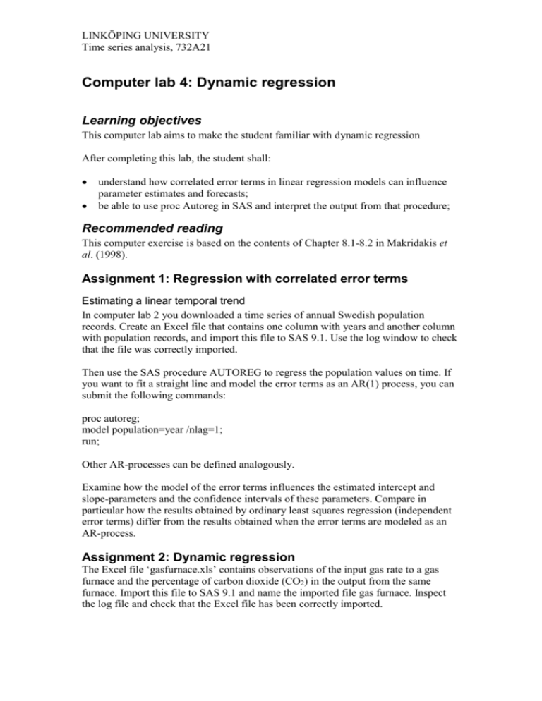
LINKÖPING UNIVERSITY
Time series analysis, 732A21
Computer lab 4: Dynamic regression
Learning objectives
This computer lab aims to make the student familiar with dynamic regression
After completing this lab, the student shall:


understand how correlated error terms in linear regression models can influence
parameter estimates and forecasts;
be able to use proc Autoreg in SAS and interpret the output from that procedure;
Recommended reading
This computer exercise is based on the contents of Chapter 8.1-8.2 in Makridakis et
al. (1998).
Assignment 1: Regression with correlated error terms
Estimating a linear temporal trend
In computer lab 2 you downloaded a time series of annual Swedish population
records. Create an Excel file that contains one column with years and another column
with population records, and import this file to SAS 9.1. Use the log window to check
that the file was correctly imported.
Then use the SAS procedure AUTOREG to regress the population values on time. If
you want to fit a straight line and model the error terms as an AR(1) process, you can
submit the following commands:
proc autoreg;
model population=year /nlag=1;
run;
Other AR-processes can be defined analogously.
Examine how the model of the error terms influences the estimated intercept and
slope-parameters and the confidence intervals of these parameters. Compare in
particular how the results obtained by ordinary least squares regression (independent
error terms) differ from the results obtained when the error terms are modeled as an
AR-process.
Assignment 2: Dynamic regression
The Excel file ‘gasfurnace.xls’ contains observations of the input gas rate to a gas
furnace and the percentage of carbon dioxide (CO2) in the output from the same
furnace. Import this file to SAS 9.1 and name the imported file gas furnace. Inspect
the log file and check that the Excel file has been correctly imported.
LINKÖPING UNIVERSITY
Time series analysis, 732A21
Run proc Autoreg with time-lagged inputs
Use proc Autotreg to regress the response variable (percentage of carbon dioxide in
the output of the gas furnace) on a suitable number of time-lagged series of the input
gasrate. Use a low order AR-process to model the noise. The SAS commands below
show how you can carry out the desired calculations, if 'gasfurnace' is the name of the
imported data set, CO2 is the name of the response variable, and gasrate, gasrate1,
gasrate2, etc. denote the input with different time lags.
data newdata;
set work.gasfurnace;
gasrate1=lag1(gasrate);
gasrate2=lag1(gasrate1);
…
run;
proc autoreg data=work.newdata;
model CO2=gasrate /nlag=1;
model CO2=gasrate gasrate1 /nlag=1;
model CO2=gasrate gasrate1 gasrate2 /nlag=1;
model CO2=gasrate gasrate1 gasrate2 gasrate3 /nlag=1;
model CO2=gasrate gasrate1 gasrate2 gasrate3 gasrate4/nlag=1;
….
output out=myoutputfile residual=myres predicted=mypred;
run;
Inspect the log file to check that the SAS code has been properly executed. Then use
the calculated AIC (or SBC) values to select a suitable number of time-lagged
variables in your regression model.
Inspect the parameter estimates in the model producing the smallest AIC value. Is
there any evidence that the system has a dead time, i.e., it takes some time until the
input influences the output? If that is the case, remove some of the time-lagged inputs
and run proc autoreg once more.
Inspect predicted values and residuals
The SAS dataset work.myoutputfile contains predicted CO2 levels (variable mypred)
and estimated error terms (variable myres) in the autoregressive model of the noise.
Export work.myoutputfile to Excel and MINITAB, and inspect the error terms. Do
they look like independent, identically distributed random numbers. If not, consider
the need for differencing the original time series of data or using a higher order ARmodel for the noise component.
Compare the performance of dynamic regression and ARIMA models
Use SAS (or Minitab) to fit an ordinary ARIMA model to the carbon dioxide
concentration. Compute the mean square prediction error and compare the result with
that obtained by dynamic regression.