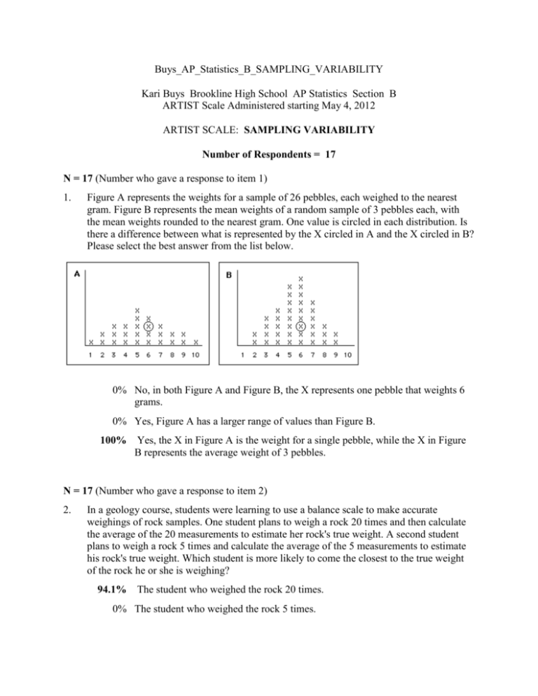
Buys_AP_Statistics_B_SAMPLING_VARIABILITY
Kari Buys Brookline High School AP Statistics Section B
ARTIST Scale Administered starting May 4, 2012
ARTIST SCALE: SAMPLING VARIABILITY
Number of Respondents = 17
N = 17 (Number who gave a response to item 1)
1.
Figure A represents the weights for a sample of 26 pebbles, each weighed to the nearest
gram. Figure B represents the mean weights of a random sample of 3 pebbles each, with
the mean weights rounded to the nearest gram. One value is circled in each distribution. Is
there a difference between what is represented by the X circled in A and the X circled in B?
Please select the best answer from the list below.
0% No, in both Figure A and Figure B, the X represents one pebble that weights 6
grams.
0% Yes, Figure A has a larger range of values than Figure B.
100%
Yes, the X in Figure A is the weight for a single pebble, while the X in Figure
B represents the average weight of 3 pebbles.
N = 17 (Number who gave a response to item 2)
2.
In a geology course, students were learning to use a balance scale to make accurate
weighings of rock samples. One student plans to weigh a rock 20 times and then calculate
the average of the 20 measurements to estimate her rock's true weight. A second student
plans to weigh a rock 5 times and calculate the average of the 5 measurements to estimate
his rock's true weight. Which student is more likely to come the closest to the true weight
of the rock he or she is weighing?
94.1%
The student who weighed the rock 20 times.
0% The student who weighed the rock 5 times.
5.9% Both averages would be equally close to the true weight.
N = 17 (Number who gave a response to item 3)
3.
Suppose half of all newborns are girls and half are boys. Hospital A, a large city hospital,
records an average of 50 births a day. Hospital B, a small, rural hospital, records an average
of 10 births a day. On a particular day, which hospital is less likely to record 80% or more
female births?
47.1%
Hospital A (with 50 births a day), because the more births you see, the closer
the proportions will be to .5.
17.6% Hospital B (with 10 births a day), because with fewer births there will be less
variability.
35.3% The two hospitals are equally likely to record such an event, because the
probability of a boy does not depend on the number of births.
N = 17 (Number who gave a response to item 4)
4.
A random sample of 25 college statistics textbook prices is obtained and the mean price is
computed. To determine the probability of finding a more extreme mean than the one
obtained from this random sample, you would need to refer to:
47.1% the population distribution of all college statistics textbook prices.
29.4% the distribution of prices for this sample of college statistics textbooks.
23.5%
the sampling distribution of textbook prices for all samples of 25 textbooks
from this population.
N = 17 (Number who gave a response to item 5)
5.
Consider the distribution of average number of hours that college students spend sleeping
each weeknight. This distribution is very skewed to the right, with a mean of 5 and a
standard deviation of 1. A researcher plans to take a simple random sample of 18 college
students. If we were to imagine that we could take all possible random samples of size 18
from the population of college students, the sampling distribution of average number of
hours spent sleeping will have a shape that is
23.5% Exactly normal.
41.2%
Less skewed than the population.
29.4% Just like the population (i.e., very skewed to the right).
5.9% It's impossible to predict the shape of the sampling distribution.
N = 17 (Number who gave a response to item 6)
6.
Imagine you have a huge jar of candies that are a generic version of M&Ms. We know that
40% of the candies in the jar are brown. Imagine that you create a sample by randomly
pulling 20 candies out of the jar. If you repeated this 10 times to create 10 samples, each
with 20 candies, about how many browns would you expect to find in each of the 10
samples?
0% Each sample would have exactly 8 brown candies.
23.5% Most of the samples would have 0 to 8 brown candies.
0% Most of the samples would have 8 to 20 brown candies.
64.7%
Most of the samples would have 6 to 10 brown candies.
11.8% You are just as likely to get any count of brown candies between 0 and 20.
Items 7 and 8 refer to the following situation:
The distribution for a population of measurements is presented below.
N = 16 (Number who gave a response to item 7)
7.
A sample of 10 randomly selected values will be taken from the population and the sample
mean will be calculated. Which of the following intervals is MOST likely to include the
sample mean?
17.6% 4 to 6
76.5%
7 to 9
0% 10 to 12
N = 17 (Number who gave a response to item 8)
8.
Another sample of 10 randomly selected values will be taken from the population and the
sample mean will be calculated. Which of the following intervals is LEAST likely to
include the sample mean?
82.4%
0 to 3
0% 4 to 7
17.6% 8 to 11
Items 9 to 14 refer to the following situation:
A hypothetical distribution for a population of test scores is displayed below. The population has
a mean of 60.4, a median of 62.8, and a standard deviation of 6.404. Each of the other four
graphs labeled A to D represent possible distributions of sample means for random samples
drawn from the population.
N = 17 (Number who gave a response to item 9)
9.
Which graph best represents a distribution of sample means for 1000 samples of size 4?
17.6% A
47.1%
B
29.4% C
5.9% D
N = 17 (Number who gave a response to item 10)
10.
What do you expect for the shape of the sampling distribution (the distribution of sample
means for all possible samples of size n = 4)?
41.2%
Shaped more like a normal distribution then like the population distribution.
52.9% Shaped more like the population distribution then like a normal distribution.
5.9% Shaped like neither the population or the normal distribution.
N = 17 (Number who gave a response to item 11)
11.
What do you expect for the variability (spread) of the sampling distribution?
17.6% Same as the population.
64.7%
Less variability than the population (a narrower distribution).
17.6% More variability than the population (a wider distribution).
N = 16 (Number who gave a response to item 12)
12.
Which graph best represents a distribution of sample means for 1000 samples of size 50?
11.8% A
5.9% B
11.8% C
64.7%
D
N = 17 (Number who gave a response to item 13)
13.
What do you expect for the shape of the sampling distribution (the distribution of sample
means for all possible samples of size n = 50)?
76.5%
Shaped more like a normal distribution.
23.5% Shaped more like the population.
0% Shaped like neither the population or the normal distribution.
N = 16 (Number who gave a response to item 14)
14.
What do you expect for the variability (spread) of the sampling distribution?
0% Same as the population.
70.6%
Less variability than the population (a narrower distribution).
23.5% More variability than the population (a wider distribution).
The distribution for a population of measurements is presented below. The mean is 3.2 and the
standard deviation is 2. Suppose that five students each take a sample of ten values from the
population and each student calculates the sample mean for his or her ten data values. The
students draw a dotplot of their five sample means on the classroom board so that they can
compare them.
N = 17 (Number who gave a response to item 15)
15.
Which of the following dotplots do you think is the most plausible for the one they drew on
the board?
11.8% a.
17.6% b.
70.6%
c.