The sorting game….
Observations:
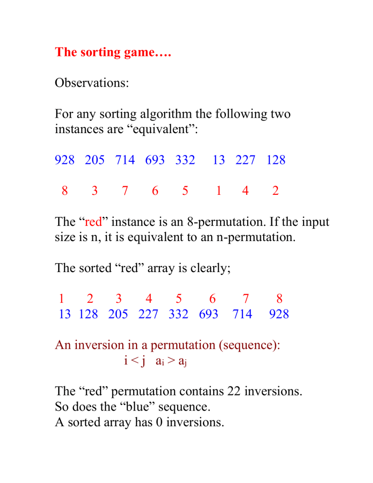
For any sorting algorithm the following two instances are “equivalent”:
928 205 714 693 332 13 227 128
8 3 7 6 5 1 4 2
The “ red ” instance is an 8-permutation. If the input size is n, it is equivalent to an n-permutation.
The sorted “red” array is clearly;
1 2 3 4 5 6 7 8
13 128 205 227 332 693 714 928
An inversion in a permutation (sequence):
i < j a i
> a j
The “red” permutation contains 22 inversions.
So does the “blue” sequence.
A sorted array has 0 inversions.

A sorting algorithm “removes” inversions.
There are n! distinct inputs for sorting an array with n objects.
The total number of inversions in all n! inputs is:

 n
2


2 n !
Hence the average number of inversions per permutation is: n(n-1)/4 = O(n 2 ).
Sorting Algorithms:
Sort the array:
928 205 714 693 332 13 227 128
944 773 374 569 207 576 725 548
761 449 726 748 585 295 194 718
BubbleSort:
928 205 714 693 332 13 227 128
944 773 374 569 207 576 725 548
761 449 726 748 585 295 194 718
205 714 693 332 13 227 128 928

773 374 569 207 576 725 548 761
449 726 748 585 295 194 718 944
205 693 332 13 227 128 714 773
374 569 207 576 725 548 761 449
726 748 585 295 194 718 928 944
The average running time of BubbleSort is O(n 2 ).
Variation: Bi-directional BubbleSort.
The average running time of BubbleSort is O(n 2 ).
SelectionSort:
928 205 714 693 332 13 227 128
944 773 374 569 207 576 725 548
761 449 726 748 585 295 194 718
928
205 928
205 714 928
205 693 714 928

Analysis: what do we count? If we use binary_search we have:
log 1 + log 2 + log 3 + …log n = log n! =
O(nlog n) comparisons.
But what about exchanges? We may have 1 + 2
+ … + n – 1 = O(n 2 ) exchanges!
MergeSort[Data, 0, 23]:
MergeSort[Data, 0, 11];
13 128 205 227 332 374 569 693
714 773 928 944
MergeSort[Data, 12, 23];
194 207 295 449 548 576 585 718
725 726 748 761
Merge[Data, 0, 23];
13 128 194 205 207 227 295 332
374 449 548 569 576 585 693 714
718 725 726 748 761 773 928 944

928 205 714 693 332 13 227 128
944 773 374 569 207 576 725 548
761 449 726 748 585 295 194 718
Analysis: How many comparisons (“cost”) does
MergeSort make?
c(n) = 2c(n/2) + (n-1)
The “cost” of “reducing” an instance of size n to two instances of size n/2 each is (n-1). The
“cost” of processing an array of size 1 is 0.
Claim: c(n) = O(nlog
2
n).
By induction; c(n)

nlog
2 n.
1.
c(1) = 0

1 .
log
2.
c(k)

klog
3.
c(n)

nlog
2
2 n.
2
1 k
 k < n
(induction hypothesis)
 c(n) = 2c(n/2) + (n – 1)
 c(n/2) = (n/2)log
2
(n/2) (induction hyp.)


2c(n/2) = n(log c(n) = n(log
2
2 n – 1) n – 1) + (n – 1)

nlog
2 n.

QuickSort[Data, 0, 23]:
Int k = SelectPivot();
928 205 714 693 332 13 227 128
944 773 374 569 207 576 725 548
761 449 726 748 585 295 194 718
Swap(Data, 0, k);
569 205 714 693 332 13 227 128
944 773 374 928 207 576 725 548
761 449 726 748 585 295 194 718 int m = Distribute(Data);
569 205 194 295 332 13 227 128
449 548 374 207 928 576 725 773
761 944 726 748 585 693 714 718
207 205 194 295 332 13 227 128
449 548 374 569 928 576 725 773
761 944 726 748 585 693 714 718

QuickSort(Data, 0, m-1);
QuickSort(Data, m+1, 23);
928 205 714 693 332 13 227 128
944 773 374 569 207 576 725 548
761 449 726 748 585 295 194 718
Analysis: Let c(n) be the “cost” (number of comparisons) the quick sort makes.
If the pivot lands in location #k then we need to:
1.
QuickSort(Data, 1, k-1);
2.
QuickSort(Data, k+1, n);
The cost of the distribution is O(n) comparisons.
This gives us the recurrence relation:
C(n) = c(k-1) + c(n-k) + n - 1
The problem we face is that we have no idea what is k. We can still do a worst case analysis.
Intuitively, this happens when the “divide & conquer” fails to properly divide the problem into two almost equal parts. In the worst case it will happen when the pivot will repeatedly end up in the first location. The above recurrence relation will then become:

c(n) = c(1) + c(n-1) + n = c(n-1) + n-1
This yields: c(n) = n-1 + (n-2) + (n-3) + … + 2 + 1 = O(n 2 ).
Average case: For each choice of the pivot, there are n possibilities: it can end up in location 1, 2,
… or n. If the pivot is chosen randomly, each one of them is equally likely. Therefore the average “cost” will be: c ( n )

1 n k n 

1 c ( k

1 )
 c ( n
 k )

( n

1 )
This is a recurrence relation. Solving it yields: c(n) = O(nlog n)
In practice, QuickSort usually beats all other sorts especially on random collections.
Definition: A sort is called STABLE if a i
= a j and i < j then in the final sort a i
will appear before a j
.
RadixSort(Data);
//Group by last digit:
761 332 693 13 773 714 944 374

194 205 725 585 295 576 726 227
207 928 128 548 748 718 569 449
//Group by next digit
205 207 13 714 718 725 726 227
928 128 332 944 548 748 449 761
569 773 374 576 585 693 194 295
//Group by next digit
13 128 194 205 207 227 295 332
374 449 548 569 576 585 693 714
718 725 726 748 761 773 928 944
RadixSort is a stable sort.
Analysis: Each scan takes n insertions. If we are doing k scans then Radix sort will execute k*n insertions or its running time is: O(n).
Odd-Even sort:
Do { for (i = 0; i < n/2; i++)
cex(A[2*i], A[2*i+1]); //Even loop for (i = 1; i < n/2; i++) cex(A[2*i-1], A[2*i]); //Odd loop
} while !sorted;

928 205 714 693 332 13 227 128
944 773 374 569 207 576 725 548
205 928 693 714 13 332 128 227
773 944 374 569 207 576 548 725
205 693 928 13 714 128 332 227
773 374 944 207 569 548 576 725
This is the array after one “phase”.
A few questions about this algorithm:
1.
Does it sort the array A?
2.
It compares adjacent entries, so its running time is O(n 2 ). So why bother?
1.
Yes it does. Let us trace the motion of the largest entry. In any “phase”, if it is not at the end of the array, it will move one or two steps to the “right”. In other words, after at most n phases it will end up at the end of the array. A similar argument applies to the second largest, third and so on. So indeed the array will be sorted.
2.
Why bother? None of the previous algorithms can take advantage of

parallelism. The “next” cex has to “wait” for the outcome of the previous. Not so for the Odd-Even sort. Indeed, in at most n parallel phases it will sort the array!