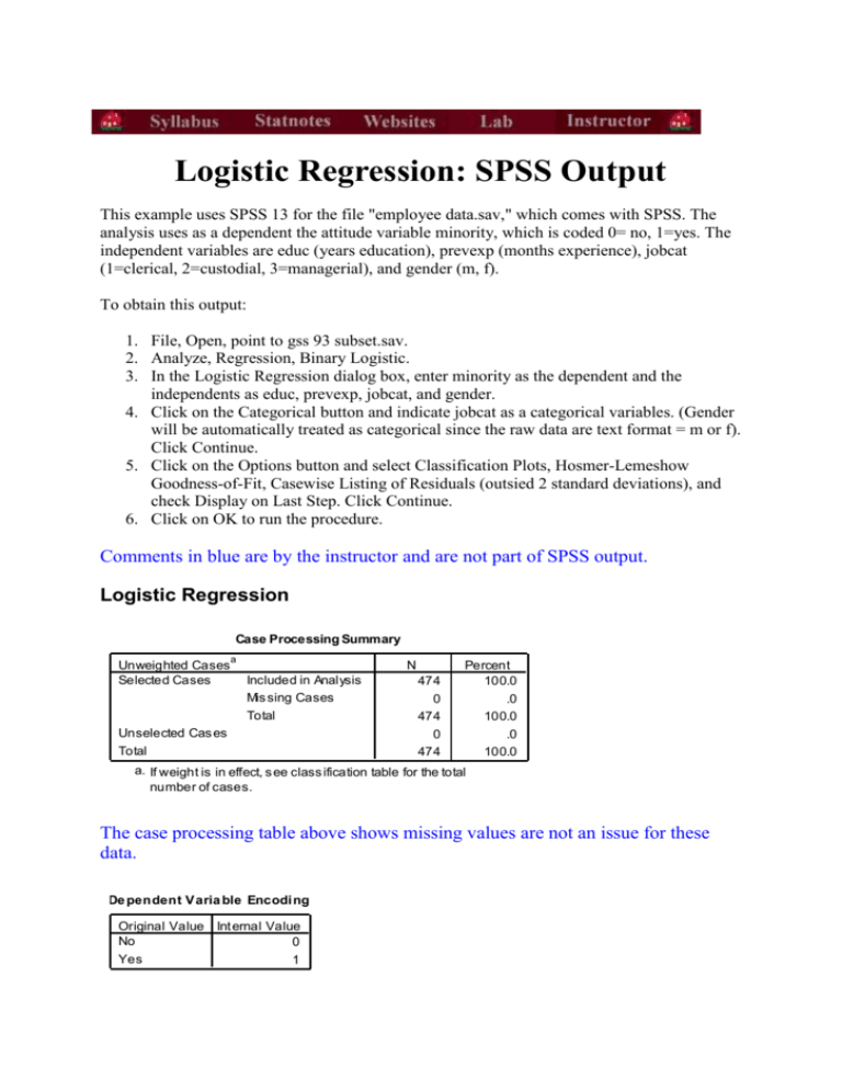
Logistic Regression: SPSS Output
This example uses SPSS 13 for the file "employee data.sav," which comes with SPSS. The
analysis uses as a dependent the attitude variable minority, which is coded 0= no, 1=yes. The
independent variables are educ (years education), prevexp (months experience), jobcat
(1=clerical, 2=custodial, 3=managerial), and gender (m, f).
To obtain this output:
1. File, Open, point to gss 93 subset.sav.
2. Analyze, Regression, Binary Logistic.
3. In the Logistic Regression dialog box, enter minority as the dependent and the
independents as educ, prevexp, jobcat, and gender.
4. Click on the Categorical button and indicate jobcat as a categorical variables. (Gender
will be automatically treated as categorical since the raw data are text format = m or f).
Click Continue.
5. Click on the Options button and select Classification Plots, Hosmer-Lemeshow
Goodness-of-Fit, Casewise Listing of Residuals (outsied 2 standard deviations), and
check Display on Last Step. Click Continue.
6. Click on OK to run the procedure.
Comments in blue are by the instructor and are not part of SPSS output.
Logistic Regression
Case Processing Summary
Unweighted Cases
Selected Cases
a
N
Included in Analysis
Mis sing Cases
Total
Unselected Cas es
Total
474
0
474
0
474
Percent
100.0
.0
100.0
.0
100.0
a. If weight is in effect, s ee class ification table for the total
number of cases.
The case processing table above shows missing values are not an issue for these
data.
De pendent Varia ble Encodi ng
Original Value Int ernal Value
No
0
Yes
1
The Dependent Variable Encoding table above shows the dependent variable,
minority, is coded with the reference category=1="yes", and the non-minority
category is coded 0. This conventional for logistic analysis, which here focuses on
the probability that minority=1.
Ca tegorical Varia ble s Codings
Employment
Category
Gender
Clerical
Custodial
Manager
Male
Female
Frequency
363
27
84
258
216
Parameter coding
(1)
(2)
1.000
.000
.000
1.000
.000
.000
1.000
.000
Above is SPSS's parameterization of the two categorical independent variables.
Note that its parameter coefficients for the last category of each such variable are
all 0's, indicating the last category is the omitted value for that set of dummy
variables. The parameter codings are the X values for the dummy variables. They
are are multiplied by the logit (effect) coefficients as part of obtaining the predicted
values of the dependent, much as one would compute an OLS regression estimate.
Block 0: Beginning Block
Classification Table a,b
Predicted
Step 0
Observed
Minority Classification
No
Yes
Overall Percentage
Minority Classification
No
Yes
370
0
104
0
Percentage
Correct
100.0
.0
78.1
a. Constant is included in the model.
b. The cut value is .500
The classification table above is a 2 x 2 table which tallies correct and incorrect
estimates for the null model with only the constant. The columns are the two
predicted values of the dependent, while the rows are the two observed (actual)
values of the dependent. In a perfect model, all cases will be on the diagonal and
the overall percent correct will be 100%. If the logistic model has homoscedasticity
(not a logistic regression assumption), the percent correct will be approximately the
same for both rows. Here it is not, with the model predicting non-minority cases
but not predicting any minority cases. While the overall percent correctly predicted
seems moderately good at 78.1%, the researcher must note that blindly estimating
the most frequent category (non-minority) for all cases would yield the same
percent correct (78.1%).
Va riables in the Equa tion
St ep 0
B
-1. 269
Constant
S. E.
.111
W ald
130.755
df
1
Sig.
.000
Ex p(B)
.281
Above SPSS prints the initial test for the model in which the coefficients for all the
independent variables are 0. The finding of significance above indicates this null
model should be rejected.
Variables not in the Equation
Step
0
Variables
Score
8.371
9.931
26.172
3.715
11.481
2.714
34.047
educ
prevexp
jobcat
jobcat(1)
jobcat(2)
gender(1)
Overall Statistics
df
1
1
2
1
1
1
5
Sig.
.004
.002
.000
.054
.001
.099
.000
Block 1: Method = Enter
Omnibus Tests of Model Coefficients
Step 1
Step
Block
Model
Chi-square
37.303
37.303
37.303
df
5
5
5
Sig.
.000
.000
.000
The chi-square goodness-of-fit test tests the null hypothesis that the step is justified.
Here the step is from the constant-only model to the all-independents model. When
as here the step was to add a variable or variables, the inclusion is justified if the
significance of the step is less than 0.05. Had the step been to drop variables from
the equation, then the exclusion would have been justified if the significance of the
change was large (ex., over 0.10).
Model Summary
Step
1
-2 Log
Cox & Snell
likelihood
R Square
461.496a
.076
Nagelkerke
R Square
.116
a. Es timation terminated at iteration number 6 because
parameter estimates changed by les s than .001.
The Cox-Snell R2 and Nagelkerke R2 are attempts to provide a logistic analogy to
R2 in OLS regression. The Nagelkerke measure adapts the Cox-Snell measure so
that it varies from 0 to 1, as does R2 in OLS.
Hosme r and Leme show Test
St ep
1
Chi-square
15.450
df
Sig.
.051
8
The Hosmer and Lemeshow Goodness-of-Fit Test divides subjects into deciles
based on predicted probabilities, then computes a chi-square from observed and
expected frequencies. The p-value=0.051 here is computed from the chi-square
distribution with 8 degrees of freedom and indicates that the logistic model is a
(barely) good fit. That is, if the Hosmer and Lemeshow Goodness-of-Fit test
statistic is .05 or less, we reject the null hypothesis that there is no difference
between the observed and predicted values of the dependent; if it is greater, as we
want, we fail to reject the null hypothesis that there is no difference, implying that
the model's estimates fit the data at an acceptable level. As here, this does not mean
that the model explains much of the variance in the dependent, only that it does so
to a significant degree.
Contingency Table for Hosmer and Lemeshow Test
Step
1
1
2
3
4
5
6
7
8
9
10
Minority Classification
= No
Observed
Expected
47
45.020
43
43.282
43
38.046
39
38.710
36
38.104
29
36.597
38
34.103
34
33.587
33
32.823
28
29.728
Minority Classification
= Yes
Observed
Expected
0
1.980
4
3.718
3
7.954
8
8.290
11
8.896
18
10.403
9
12.897
13
13.413
14
14.177
24
22.272
Total
47
47
46
47
47
47
47
47
47
52
Classification Table a
Predicted
Step 1
Observed
Minority Classification
Overall Percentage
No
Yes
Minority Classification
No
Yes
363
7
103
1
Percentage
Correct
98.1
1.0
76.8
a. The cut value is .500
The classification table above is a 2 x 2 table which tallies correct and incorrect
estimates for the full model with the independents as well as the constant. The
columns are the two predicted values of the dependent, while the rows are the two
observed (actual) values of the dependent. In a perfect model, all cases will be on
the diagonal and the overall percent correct will be 100%. If the logistic model has
homoscedasticity (not a logistic regression assumption), the percent correct will be
approximately the same for both rows. Here it is not, with the model predicting all
but seven non-minority cases but predicting only one minority cases. While the
overall percent correctly predicted seems moderately good at 76.8%, the researcher
must note that blindly estimating the most frequent category (non-minority) for all
cases would yield an even higher percent correct (78.1%), as noted above. This
implies minority status cannot be differentiated on the basis of education, job
experience, job category, and gender for these data.
Variables in the Equation
Step
a
1
educ
prevexp
jobcat
jobcat(1)
jobcat(2)
gender(1)
Constant
B
-.008
.002
S.E.
.054
.001
2.048
2.456
.579
-3.523
.572
.765
.262
1.040
Wald
.020
1.913
13.417
12.803
10.313
4.868
11.473
df
1
1
2
1
1
1
1
Sig.
.886
.167
.001
.000
.001
.027
.001
Exp(B)
.992
1.002
7.755
11.662
1.784
.030
a. Variable(s) entered on s tep 1: educ, prevexp, jobcat, gender.
The Wald statistic above and the corresponding significance level test the
significance of each of the covariate and dummy independents in the model. The
ratio of the logistic coefficient B to its standard error S.E., squared, equals the Wald
statistic. If the Wald statistic is significant (i.e., less than 0.05) then the parameter is
significant in the model. Of the independents, jobcat and gender are significant but
educ and prevexp are not.
The "Exp(b)" column is SPSS's label for the odds ratio of the row independent with
the dependent (minority).It is the predicted change in odds for a unit increase in the
corresponding independent variable. Odds ratios less than 1 correspond to
decreases and odds ratios more than 1.0 correspond to increases in odds. Odds
ratios close to 1.0 indicate that unit changes in that independent variable do not
affect the dependent variable.
Step number: 1
Observed Groups and Predicted Probabilities
F
R
E
Q
U
E
160 



120 



80 
Y
N
N
N










N


N
YY

 N
N
NN

40  N
NY
NN

 N
NN
NN

 NN
NNYN NNY

 NNN
NNNNY NNNYY Y Y
Y Y

Predicted


Prob:
0
.25
.5
.75
1
Group: NNNNNNNNNNNNNNNNNNNNNNNNNNNNNNYYYYYYYYYYYYYYYYYYYYYYYYYYYYYY
N
C
Y
Predicted Probability is of Membership for Yes
The Cut Value is .50
Symbols: N - No
Y - Yes
Each Symbol Represents 10 Cases.
The classplot above is an alternative way of assessing correct and incorrect
predictions under logistic regression. The X axis is the predicted probability from
0.0 to 1.0 of the dependent being classified "1" (minority status). The Y axis is
frequency: the number of cases classified. Inside the plot are columns of observed
1's and 0's, which it here codes as Y's (for minority status) and N's (not minority),
with 10 cases per symbol. Examining this plot will tell such things as how well the
model classifies difficult cases (ones near p = .5). In this case, it also shows nearly
all cases are coded as being in the N (not minority status) group, even if in reality
they are in the Y (minority) group.
http://faculty.chass.ncsu.edu/garson/PA765/logispss.htm