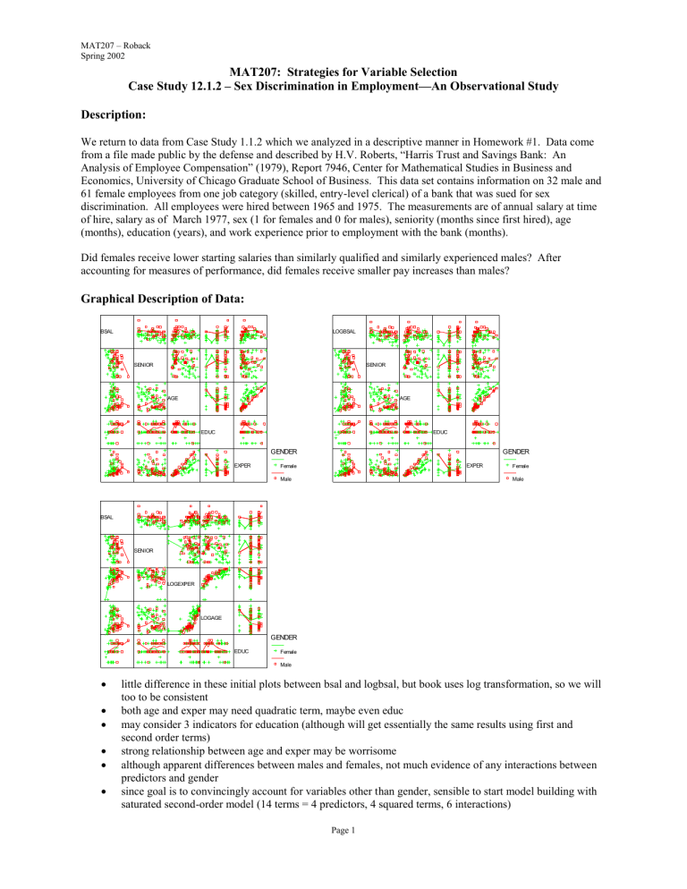
MAT207 – Roback
Spring 2002
MAT207: Strategies for Variable Selection
Case Study 12.1.2 – Sex Discrimination in Employment—An Observational Study
Description:
We return to data from Case Study 1.1.2 which we analyzed in a descriptive manner in Homework #1. Data come
from a file made public by the defense and described by H.V. Roberts, “Harris Trust and Savings Bank: An
Analysis of Employee Compensation” (1979), Report 7946, Center for Mathematical Studies in Business and
Economics, University of Chicago Graduate School of Business. This data set contains information on 32 male and
61 female employees from one job category (skilled, entry-level clerical) of a bank that was sued for sex
discrimination. All employees were hired between 1965 and 1975. The measurements are of annual salary at time
of hire, salary as of March 1977, sex (1 for females and 0 for males), seniority (months since first hired), age
(months), education (years), and work experience prior to employment with the bank (months).
Did females receive lower starting salaries than similarly qualified and similarly experienced males? After
accounting for measures of performance, did females receive smaller pay increases than males?
Graphical Description of Data:
BSAL
LOGBSAL
SENIOR
SENIOR
AGE
AGE
EDUC
EDUC
GENDER
EXPER
GENDER
EXPER
Female
Male
Female
Male
BSAL
SENIOR
LOGEXPER
LOGAGE
GENDER
EDUC
Female
Male






little difference in these initial plots between bsal and logbsal, but book uses log transformation, so we will
too to be consistent
both age and exper may need quadratic term, maybe even educ
may consider 3 indicators for education (although will get essentially the same results using first and
second order terms)
strong relationship between age and exper may be worrisome
although apparent differences between males and females, not much evidence of any interactions between
predictors and gender
since goal is to convincingly account for variables other than gender, sensible to start model building with
saturated second-order model (14 terms = 4 predictors, 4 squared terms, 6 interactions)
Page 1
MAT207 – Roback
Spring 2002
Saturated Second-order Model:




must Transform…Compute all squared terms and interactions (ugh!)
when doing Analyze…Regression…Linear, it helps to move all candidate predictors to end of spreadsheet
correlation table from Analyze…Correlate…Bivariate
VIFs in Coefficients table from selecting Collinearity Diagnostics under Statistics in Linear Regression
.3
.2
.1
Model
1
R
.705a
R Square
.497
Unstandardized Residual
Model Summaryb
Adjusted
R Square
.407
Std. Error of
the Estimate
9.949E-02
a. Predictors: (Constant), EDUBYEXP, SENIOR2, EDUC,
AGE, EXPER2, SENBYEXP, AGEBYEDU, SENBYEDU,
EDUC2, SENBYAGE, AGEBYEXP, AGE2, SENIOR,
EXPER
-.0
-.1
-.2
-.3
8.3
b. Dependent Variable: LOGBSAL
8.4
8.5
8.6
8.7
8.8
8.9
Unstandardized Pr edicted V alue
Correlations
LOGBSAL
SENIOR
AGE
EDUC
EXPER
Pearson Correlation
Sig. (2-tailed)
N
Pearson Correlation
Sig. (2-tailed)
N
Pearson Correlation
Sig. (2-tailed)
N
Pearson Correlation
Sig. (2-tailed)
N
Pearson Correlation
Sig. (2-tailed)
N
LOGBSAL
1.000
.
93
-.294**
.004
93
.065
.537
93
.407**
.000
93
.188
.071
93
SENIOR
-.294**
.004
93
1.000
.
93
-.184
.077
93
.060
.569
93
-.075
.477
93
AGE
.065
.537
93
-.184
.077
93
1.000
.
93
-.225*
.030
93
.798**
.000
93
EDUC
.407**
.000
93
.060
.569
93
-.225*
.030
93
1.000
.
93
-.101
.335
93
EXPER
.188
.071
93
-.075
.477
93
.798**
.000
93
-.101
.335
93
1.000
.
93
**. Correlation is significant at the 0.01 level (2-tailed).
*. Correlation is significant at the 0.05 level (2-tailed).
Coefficientsa
Model
1
(Constant)
SENIOR
AGE
EDUC
EXPER
SENIOR2
AGE2
EDUC2
EXPER2
SENBYAGE
SENBYEDU
SENBYEXP
AGEBYEDU
AGEBYEXP
EDUBYEXP
Unstandardized
Coefficients
B
Std. Error
6.835
1.340
2.678E-02
.022
1.717E-04
.002
7.995E-02
.078
3.376E-03
.003
-1.33E-04
.000
9.425E-07
.000
1.388E-03
.002
-1.59E-06
.000
-3.55E-06
.000
-5.99E-04
.000
1.090E-05
.000
-6.98E-05
.000
-3.72E-06
.000
-7.50E-05
.000
Standardi
zed
Coefficien
ts
Beta
2.125
.186
1.412
2.376
-1.718
1.030
.590
-.361
-.320
-1.080
.656
-.998
-1.836
-.651
t
5.102
1.218
.073
1.023
1.048
-1.128
.542
.741
-.481
-.242
-1.219
.442
-1.087
-.880
-.876
Sig.
.000
.227
.942
.310
.298
.263
.589
.461
.632
.809
.227
.660
.281
.382
.384
95% Confidence Interval for B
Lower Bound
Upper Bound
4.168
9.502
-.017
.071
-.005
.005
-.076
.236
-.003
.010
.000
.000
.000
.000
-.002
.005
.000
.000
.000
.000
-.002
.000
.000
.000
.000
.000
.000
.000
.000
.000
Collinearity Statistics
Tolerance
VIF
.002
.001
.003
.001
.003
.002
.010
.011
.004
.008
.003
.008
.001
.012
472.164
1012.083
295.800
798.235
359.564
559.476
98.346
87.244
271.041
121.765
342.055
130.870
675.285
85.736
a. Dependent Variable: LOGBSAL

residual plot looks fine, but high VIFs and lack of significance of any predictors indicates there’s problems
with multicollinearity
Identifying Good Subset Models:

Analyze…Regression…Linear. Dependent = logbsal; independent(s) = all 14 candidates; Method = stepwise or
backward or forward (can set criteria under Options)
Page 2
MAT207 – Roback
Spring 2002
a) Stepwise
Variables Entered/Removeda
Model
1
Variables
Entered
Variables
Removed
EDUC2
.
SENBYED
U
.
SENBYEX
P
.
AGEBYEX
P
.
EXPER
.
Model Summary
Model
1
2
3
4
5
6
7
R
.422a
.535b
.574c
.616d
.645e
.645f
.680g
R Square
.178
.287
.329
.379
.415
.415
.462
Adjusted
R Square
.169
.271
.306
.351
.382
.389
.431
Std. Error of
the Estimate
.1178
.1103
.1076
.1041
.1016
.1010
9.747E-02
2
3
4
a. Predictors: (Constant), EDUC2
b. Predictors: (Constant), EDUC2, SENBYEDU
5
c. Predictors: (Constant), EDUC2, SENBYEDU,
SENBYEXP
d. Predictors: (Constant), EDUC2, SENBYEDU,
SENBYEXP, AGEBYEXP
e. Predictors: (Constant), EDUC2, SENBYEDU,
SENBYEXP, AGEBYEXP, EXPER
6
.
7
EDUBYEX
P
f. Predictors: (Constant), EDUC2, SENBYEDU,
AGEBYEXP, EXPER
g. Predictors: (Constant), EDUC2, SENBYEDU,
AGEBYEXP, EXPER, EDUBYEXP
SENBYEX
P
.
Method
Stepwise (Criteria:
Probability-of-F-to-enter <= .050,
Probability-of-F-to-remove >= .100).
Stepwise (Criteria:
Probability-of-F-to-enter <= .050,
Probability-of-F-to-remove >= .100).
Stepwise (Criteria:
Probability-of-F-to-enter <= .050,
Probability-of-F-to-remove >= .100).
Stepwise (Criteria:
Probability-of-F-to-enter <= .050,
Probability-of-F-to-remove >= .100).
Stepwise (Criteria:
Probability-of-F-to-enter <= .050,
Probability-of-F-to-remove >= .100).
Stepwise (Criteria:
Probability-of-F-to-enter <= .050,
Probability-of-F-to-remove >= .100).
Stepwise (Criteria:
Probability-of-F-to-enter <= .050,
Probability-of-F-to-remove >= .100).
a. Dependent Variable: LOGBSAL
b) Backward
c) Forward
Model Summary
Model
1
2
3
4
5
6
7
8
9
R
.705a
.705b
.705c
.704d
.704e
.702f
.698g
.695h
.692i
R Square
.497
.497
.497
.496
.495
.492
.487
.484
.479
Adjusted
R Square
.407
.415
.421
.427
.433
.437
.438
.441
.442
Std. Error of
the Estimate
9.949E-02
9.886E-02
9.828E-02
9.778E-02
9.726E-02
9.692E-02
9.684E-02
9.659E-02
9.648E-02
a. Predictors: (Constant), EDUBYEXP, SENIOR2, EDUC,
AGE, EXPER2, SENBYEXP, AGEBYEDU, SENBYEDU,
EDUC2, SENBYAGE, AGEBYEXP, AGE2, SENIOR,
EXPER
b. Predictors: (Constant), EDUBYEXP, SENIOR2, EDUC,
EXPER2, SENBYEXP, AGEBYEDU, SENBYEDU,
EDUC2, SENBYAGE, AGEBYEXP, AGE2, SENIOR,
EXPER
c. Predictors: (Constant), EDUBYEXP, SENIOR2, EDUC,
EXPER2, SENBYEXP, AGEBYEDU, SENBYEDU,
EDUC2, AGEBYEXP, AGE2, SENIOR, EXPER
d. Predictors: (Constant), EDUBYEXP, SENIOR2, EDUC,
EXPER2, AGEBYEDU, SENBYEDU, EDUC2,
AGEBYEXP, AGE2, SENIOR, EXPER
e. Predictors: (Constant), EDUBYEXP, SENIOR2, EDUC,
AGEBYEDU, SENBYEDU, EDUC2, AGEBYEXP, AGE2,
SENIOR, EXPER
f. Predictors: (Constant), EDUBYEXP, SENIOR2, EDUC,
AGEBYEDU, SENBYEDU, AGEBYEXP, AGE2, SENIOR,
EXPER
g. Predictors: (Constant), EDUBYEXP, EDUC,
AGEBYEDU, SENBYEDU, AGEBYEXP, AGE2, SENIOR,
EXPER
h. Predictors: (Constant), EDUBYEXP, EDUC,
AGEBYEDU, SENBYEDU, AGEBYEXP, AGE2, EXPER
i. Predictors: (Constant), EDUC, AGEBYEDU,
SENBYEDU, AGEBYEXP, AGE2, EXPER
Model Summary
Model
1
2
3
4
5
6
R
R Square
.422a
.178
b
.535
.287
.574c
.329
d
.616
.379
.645e
.415
f
.680
.463
Adjusted
R Square
.169
.271
.306
.351
.382
.425
Std. Error of
the Estimate
.1178
.1103
.1076
.1041
.1016
9.795E-02
a. Predictors: (Constant), EDUC2
b. Predictors: (Constant), EDUC2, SENBYEDU
c. Predictors: (Constant), EDUC2, SENBYEDU,
SENBYEXP
d. Predictors: (Constant), EDUC2, SENBYEDU,
SENBYEXP, AGEBYEXP
e. Predictors: (Constant), EDUC2, SENBYEDU,
SENBYEXP, AGEBYEXP, EXPER
f. Predictors: (Constant), EDUC2, SENBYEDU,
SENBYEXP, AGEBYEXP, EXPER, EDUBYEXP
Page 3
MAT207 – Roback
Spring 2002
a-c) Create a model based on sequential variable selection techniques (honoring rule to include
linear terms whenever those terms are used in quadratic or interaction terms):
Model Summary
Model
1
R
.681a
Adjusted
R Square
.413
R Square
.464
Std. Error of
the Estimate
9.903E-02
a. Predictors: (Constant), EDUBYEXP, SENIOR, EDUC,
AGE, AGEBYEXP, EXPER, EDUC2, SENBYEDU
Coefficientsa
Model
1
(Constant)
SENIOR
AGE
EDUC
EXPER
EDUC2
SENBYEDU
AGEBYEXP
EDUBYEXP
Unstandardized
Coefficients
B
Std. Error
8.148
.561
1.899E-03
.006
4.928E-05
.000
2.678E-02
.056
4.506E-03
.001
1.845E-03
.002
-4.21E-04
.000
-3.75E-06
.000
-1.40E-04
.000
Standardi
zed
Coefficien
ts
Beta
.151
.053
.473
3.172
.784
-.760
-1.849
-1.217
t
14.512
.344
.348
.476
4.781
1.082
-.972
-3.604
-2.669
Sig.
.000
.731
.729
.636
.000
.282
.334
.001
.009
95% Confidence Interval for B
Lower Bound
Upper Bound
7.031
9.264
-.009
.013
.000
.000
-.085
.139
.003
.006
-.002
.005
-.001
.000
.000
.000
.000
.000
Collinearity Statistics
Tolerance
VIF
.033
.271
.006
.015
.012
.010
.024
.031
30.011
3.696
154.977
68.952
82.240
95.698
41.232
32.548
a. Dependent Variable: LOGBSAL
Collinearity Diagnosticsa
Model
1
Dimension
1
2
3
4
5
6
7
8
9
Eigenvalue
7.774
1.052
.117
2.908E-02
1.335E-02
1.034E-02
4.032E-03
4.770E-04
9.607E-05
Condition
Index
1.000
2.719
8.138
16.350
24.134
27.415
43.910
127.656
284.463
(Constant)
.00
.00
.00
.00
.00
.01
.01
.00
.98
SENIOR
.00
.00
.00
.01
.00
.00
.00
.26
.74
AGE
.00
.00
.04
.31
.07
.37
.15
.00
.07
EDUC
.00
.00
.00
.00
.00
.00
.00
.10
.90
Variance Proportions
EXPER
EDUC2
.00
.00
.00
.00
.00
.00
.00
.00
.00
.01
.10
.00
.83
.00
.01
.74
.06
.24
SENBYEDU
.00
.00
.00
.00
.00
.01
.01
.25
.73
AGEBYEXP
.00
.00
.00
.00
.40
.03
.56
.00
.00
EDUBYEXP
.00
.00
.02
.00
.43
.01
.36
.00
.17
a. Dependent Variable: LOGBSAL

some guidelines suggest VIF>10 or Condition Index>30 imply possible problems with multicollinearity
d) Book’s Model (Section 12.6):

Analyze…Regression…Linear. Dependent = logbsal; independent(s) = first enter all 4 main effects and hit Next
to identify Block 1, then enter remaining 10 predictors as Block 2; Method = stepwise
.3
.2
Model Summ ary
R
R Square
.568a
.322
.635b
.403
.685c
.469
Adjust ed
R Square
.292
.369
.431
Unstandardized Residual
Model
1
2
3
St d. Error of
the Es timate
.1088
.1026
9.743E-02
.1
-.0
-.1
a. Predic tors: (Constant), EXPER, SENIOR, EDUC, AGE
b. Predic tors: (Constant), EXPER, SENIOR, EDUC, AGE,
AGEBYEXP
c. Predic tors: (Constant), EXPER, SENIOR, EDUC, AGE,
AGEBYEXP, AGEBYEDU
-.2
-.3
8.3
8.4
8.5
Unstandardized Pr edicted V alue
Page 4
8.6
8.7
8.8
MAT207 – Roback
Spring 2002
Coefficientsa
Model
1
2
3
(Constant)
SENIOR
AGE
EDUC
EXPER
(Constant)
SENIOR
AGE
EDUC
EXPER
AGEBYEXP
(Constant)
SENIOR
AGE
EDUC
EXPER
AGEBYEXP
AGEBYEDU
Unstandardized
Coefficients
B
Std. Error
8.658
.139
-4.12E-03
.001
-1.66E-04
.000
2.388E-02
.005
4.972E-04
.000
8.567
.134
-3.70E-03
.001
1.352E-05
.000
2.004E-02
.005
2.813E-03
.001
-3.69E-06
.000
7.887
.245
-3.15E-03
.001
1.241E-03
.000
7.203E-02
.017
2.856E-03
.001
-3.72E-06
.000
-1.02E-04
.000
Standardi
zed
Coefficien
ts
Beta
t
62.338
-3.631
-1.173
4.641
2.365
64.057
-3.435
.095
4.022
4.007
-3.439
32.214
-3.041
3.090
4.315
4.284
-3.655
-3.247
-.327
-.180
.422
.350
-.293
.015
.354
1.980
-1.818
-.250
1.347
1.272
2.010
-1.834
-1.464
Sig.
.000
.000
.244
.000
.020
.000
.001
.925
.000
.000
.001
.000
.003
.003
.000
.000
.000
.002
95% Confidence Interval for B
Lower Bound
Upper Bound
8.382
8.934
-.006
-.002
.000
.000
.014
.034
.000
.001
8.301
8.832
-.006
-.002
.000
.000
.010
.030
.001
.004
.000
.000
7.400
8.373
-.005
-.001
.000
.002
.039
.105
.002
.004
.000
.000
.000
.000
Collinearity Statistics
Tolerance
VIF
.951
.328
.932
.352
1.051
3.045
1.073
2.844
.939
.285
.885
.028
.025
1.065
3.511
1.130
35.610
40.755
.914
.033
.071
.028
.025
.030
1.094
30.735
14.073
35.624
40.759
32.902
a. Dependent Variable: LOGBSAL
Collinearity Diagnosticsa
Model
1
2
3
Dimension
1
2
3
4
5
1
2
3
4
5
6
1
2
3
4
5
6
7
Eigenvalue
4.556
.386
3.387E-02
2.014E-02
4.600E-03
5.226
.708
3.388E-02
2.043E-02
6.720E-03
4.279E-03
6.193
.713
4.508E-02
3.383E-02
8.379E-03
5.925E-03
5.995E-04
Condition
Index
1.000
3.437
11.597
15.040
31.471
1.000
2.716
12.419
15.995
27.887
34.947
1.000
2.947
11.721
13.530
27.186
32.330
101.639
(Constant)
.00
.00
.00
.01
.99
.00
.00
.00
.01
.06
.93
.00
.00
.00
.00
.05
.02
.92
SENIOR
.00
.00
.00
.36
.64
.00
.00
.00
.36
.04
.60
.00
.00
.09
.00
.60
.21
.10
Variance Proportions
AGE
EDUC
EXPER
.00
.00
.01
.00
.01
.30
.42
.32
.40
.22
.44
.14
.36
.24
.16
.00
.00
.00
.00
.01
.00
.37
.30
.03
.20
.38
.00
.00
.21
.86
.43
.10
.10
.00
.00
.00
.00
.00
.00
.00
.00
.00
.04
.02
.03
.01
.01
.21
.00
.03
.75
.94
.94
.00
AGEBYEXP
AGEBYEDU
.00
.01
.00
.01
.80
.19
.00
.01
.00
.00
.16
.83
.00
.00
.00
.03
.00
.03
.01
.92
a. Dependent Variable: LOGBSAL

note that even this model is not immune from multicollinearity issues. However, removing any of these
predictors significantly affects performance, plus we’re not planning prediction and we don’t seem to have
extremely high standard errors of coefficients
Details of Stepwise procedure:
Variables Entered/Removedb
Model
1
2
3
Variabl es
Entered
EXPER,
SENIOR,
a
EDUC, AGE
AGEBYEXP
AGEBYEDU
Variabl es
Removed
Method
.
Enter
.
.
Stepwi se (Criteria: Probability-of-F-to-enter <= .050, Probability-of-F-to-remove >= .100).
Stepwi se (Criteria: Probability-of-F-to-enter <= .050, Probability-of-F-to-remove >= .100).
a. All requested variables entered.
b. Dependent Vari able: LOGBSAL
Page 5
MAT207 – Roback
Spring 2002
Excluded Variablesd
Model
1
SENIOR2
AGE2
EDUC2
EXPER2
SENBYAGE
SENBYEDU
SENBYEXP
AGEBYEDU
AGEBYEXP
EDUBYEXP
SENIOR2
AGE2
EDUC2
EXPER2
SENBYAGE
SENBYEDU
SENBYEXP
AGEBYEDU
EDUBYEXP
SENIOR2
AGE2
EDUC2
EXPER2
SENBYAGE
SENBYEDU
SENBYEXP
EDUBYEXP
2
3
Beta In
-1.101a
-1.494a
1.178a
-.938a
.221a
-.310a
-.072a
-1.448a
-1.818a
-1.061a
-.868b
2.428b
1.078b
-.279b
.083b
-.092b
-.109b
-1.464b
-1.169b
-1.023c
1.138c
.413c
-.187c
.158c
-1.149c
.086c
-.319c
t
-.711
-1.908
1.515
-3.175
.301
-.378
-.093
-3.005
-3.439
-2.303
-.592
1.744
1.466
-.485
.119
-.118
-.149
-3.247
-2.713
-.737
.803
.557
-.341
.239
-1.457
.124
-.498
Sig.
.479
.060
.133
.002
.764
.707
.926
.003
.001
.024
.555
.085
.146
.629
.905
.906
.882
.002
.008
.463
.424
.579
.734
.811
.149
.902
.620
Collinearity Stati stics
Minimum
VIF
Tolerance
309.695
3.229E-03
82.072
1.218E-02
79.752
1.242E-02
12.501
5.519E-02
69.314
1.443E-02
86.961
1.150E-02
76.609
1.229E-02
32.899
3.040E-02
40.755
2.454E-02
28.920
3.393E-02
310.381
3.222E-03
289.243
3.457E-03
79.881
1.242E-02
47.725
6.427E-03
69.552
1.438E-02
87.557
1.142E-02
76.625
8.645E-03
32.902
2.453E-02
29.050
1.504E-02
310.748
3.218E-03
323.359
2.791E-03
88.299
7.993E-03
47.857
6.411E-03
69.639
1.109E-02
101.874
9.380E-03
77.208
8.612E-03
65.785
9.676E-03
Partial
Correlation
-.076
-.200
.160
-.322
.032
-.040
-.010
-.307
-.346
-.240
-.064
.185
.156
-.052
.013
-.013
-.016
-.330
-.281
-.080
.087
.060
-.037
.026
-.156
.013
-.054
Tolerance
3.229E-03
1.218E-02
1.254E-02
7.999E-02
1.443E-02
1.150E-02
1.305E-02
3.040E-02
2.454E-02
3.458E-02
3.222E-03
3.457E-03
1.252E-02
2.095E-02
1.438E-02
1.142E-02
1.305E-02
3.039E-02
3.442E-02
3.218E-03
3.093E-03
1.133E-02
2.090E-02
1.436E-02
9.816E-03
1.295E-02
1.520E-02
a. Predictors i n the Model: (Cons tant), EXPER, SENIOR, EDUC, AGE
b. Predictors i n the Model: (Cons tant), EXPER, SENIOR, EDUC, AGE, AGEBYEXP
c. Predictors i n the Model: (Cons tant), EXPER, SENIOR, EDUC, AGE, AGEBYEXP, AGEBYEDU
d. Dependent Variable: LOGBSAL
Book's model: Resid plot vs. Age
.3
.3
.2
.2
.1
Unstandardized Residual
.1
-.0
-.1
-.2
-.3
200
300
400
500
-.0
-.1
-.2
-.3
600
700
800
-.2
A GE

0.0
.2
.4
.6
.8
1.0
1.2
GENDER
can plot residuals against variables in the model (left) to see if a different form of that variable is needed
(turns out Age squared does not help), or against variables not in the model (right) to see if those variables
should be added
Final Model (add Gender into best subset model):
b
Model Summ ary
Model
1
R
.773a
R Square
.598
Adjust ed
R Square
.564
St d. E rror of
the Es timate
8.528E -02
a. Predic tors: (Constant), GE NDE R, E XPE R, SENIOR,
EDUC, AGE, A GE BYE DU, AGEBY EXP
b. Dependent Variable: LOGB SAL
Coeffi cientsa
Model
1
Unstandardized
Coeffic ients
B
St d. E rror
(Const ant)
8.278
.227
SE NIOR
-3. 48E -03
.001
AGE
9.147E -04
.000
EDUC
4.235E -02
.016
EXPER
2.181E -03
.001
AGEB YEDU -5. 46E -05
.000
AGEB YEXP -3. 23E -06
.000
GE NDER
-.120
.023
St andardi
zed
Coeffic ien
ts
Beta
-.276
.993
.748
1.535
-.780
-1. 594
-.442
t
36.460
-3. 830
2.562
2.700
3.650
-1. 876
-3. 608
-5. 219
Sig.
.000
.000
.012
.008
.000
.064
.001
.000
95% Confidenc e Int erval for B
Lower Bound
Upper Bound
7.827
8.729
-.005
-.002
.000
.002
.011
.074
.001
.003
.000
.000
.000
.000
-.165
-.074
a. Dependent Variable: LOGB SAL

although some high leverages, no real problems with influential points
Page 6
Collinearity Statisti cs
Tolerance
VIF
.910
.032
.062
.027
.027
.024
.660
1.099
31.707
16.205
37.372
36.529
41.207
1.515