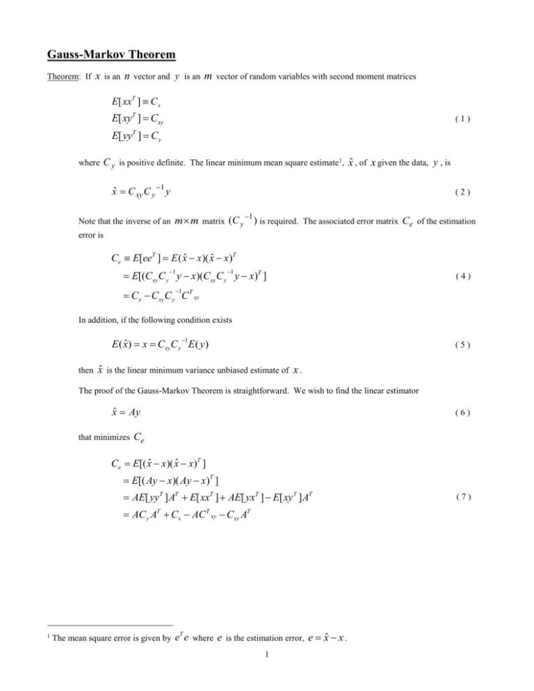
Gauss-Markov Theorem
Theorem: If
x is an n vector and y is an m vector of random variables with second moment matrices
E[ xxT ]  Cx
E[ xyT ]  Cxy
(1)
E[ yyT ]  Cy
where C y is positive definite. The linear minimum mean square estimate 1,
x̂ , of x given the data, y , is
xˆ  C xy C y 1 y
Note that the inverse of an
(2)
m m matrix (C y 1 ) is required. The associated error matrix Ce of the estimation
error is
Ce  E[eeT ]  E ( xˆ  x)( xˆ  x)T
1
1
 E[(Cxy C y y  x)(Cxy C y y  x)T ]
(4)
1
 Cx  Cxy C y C T xy
In addition, if the following condition exists
1
E ( xˆ )  x  Cxy C y E ( y)
then
(5)
x̂ is the linear minimum variance unbiased estimate of x .
The proof of the Gauss-Markov Theorem is straightforward. We wish to find the linear estimator
xˆ  Ay
that minimizes
(6)
Ce
Ce  E[( xˆ  x)( xˆ  x)T ]
 E[( Ay  x)( Ay  x)T ]
 AE[ yyT ] AT  E[ xxT ]  AE[ yxT ]  E[ xyT ] AT
 AC y AT  Cx  AC T xy  Cxy AT
1
T
The mean square error is given by e e where
e is the estimation error, e  xˆ  x .
1
(7)
Ce is found by taking the variation with respect to A
The minimum of
 Ce  0   ACy AT   ACT xy  ACy AT  Cxy AT
  A(Cy AT  CT xy )  ( ACy  Cxy ) AT  0
For arbitrary
A
(8)
this requires that
AC y  C xy  0
or,
A  C xy C y 1
i.e.
xˆ  C xy C y 1 y
For
(9)
x̂ to be unbiased
1
E ( xˆ )  x  Cxy C y E ( y)
( 10 )
Some other properties of minimum mean square error linear estimators
In two dimensions we expect
x̂ to be the true value of x projected into the y plane.
y3
x
e
y2
x̂
y1
The error vector
( e) n 1 is perpendicular to the measurement space defined by y i.e.
e  xˆ  x
To show this, multiply
( 11 )
e by y T and take the expected value
ey T  xˆy T  xyT
ˆ T ]  E[ xyT ]
E[eyT ]  E[ xy
( 12 )
2
But,
1
ˆ T ]  E[Cxy C y yyT ]
E[ xy
( 13 )
1
 C xy C y C y  C xy
Hence,
E[eyT ]  Cxy  Cxy  0
( 14 )
Also, this means that
Cexˆ  0
i.e.
( 15 )
x̂ is orthogonal to e as seen in the figure. To demonstrate this we can show that E[exˆT ]  0 as follows:
E[exˆT ]  E[( xˆ  x) xˆT ]
ˆ ˆ T ]  E[ xxˆ T ]
 E[ xx
1
1
1
 Cxy C y E[ yy T ]C y C T xy  E[ xy T ]C y C T xy
1
1
 Cxy C y C T xy  Cxy C y C T xy
0
Special Cases of the Gauss-Markov Theorem
Assume that we have a linear observation/state relationship. Then
y  Hx  
where H is an
( 16 )
m n matrix. From equation (2)
1
xˆ  Cxy C y y
( 17 )
We can compute C xy and C y , i.e.
Cxy  E[ xyT ]  E[ x( Hx   )T ]
 E[ xxT ]H T  E[ x T ]
( 18 )
 Cx H T  Cx
3
and C y
Cy  E[ yyT ]
 E[( Hx   )( Hx   )T ]
( 19 )
 HE[ xxT ]H T  HE[ x T ]  E[ xT ]H T  E[ T ]
 HCx H T  HCx  C T x H T  C
Substituting into equation (17), the estimate for
x̂ becomes
xˆ  (Cx H T  Cx )( HCx H T  HCx  C T x H T  C ) 1 y
Using the expression for
( 20 )
Ce from the Gauss-Markov Theorem
1
Ce  Cx  Cxy C y C T xy
Ce  Cx  (Cx H T  Cx )( HCx H T  HCx  C T x H T  C ) 1 (C x H T  C x )T
Note that in the case of linear observations we require knowledge of
( 21 )
C x , Cx and C in addition to the data y .
The computation of these matrices can be a difficult task. Usually we would assume that
C x is diagonal with large
diagonal elements which implies nothing is known about the true state. If we know the joint density function,
f ( x1 , x2 xn ) , then C x can be computed from its definition
 
Cx 
   xx
 
If we know

T
f ( x1 , x2
xn )dx1 , dx2
dxn
( 22 )

COV ( x)  E[( x  x )( x  x )T ] , where x is the mean of x , we can compute C x
Cx  COV ( x)  xx T
( 23 )
As stated, we generally use a diagonal matrix with large numerical values for
4
Cx .
If we have information on the joint density function, g , of the components of
 
Cx 

   x
 


  

g ( x1
xn , 1
 m )dx1
dxn d 1
d m
( 24 )

The second moment matrix,
Ce 
T
x and  , then
T
Ce , is usually assumed known, where
h(1
 m ) d 1
d m
( 25 )

, are uncorrelated2, then
If the state vector, x, and observation noise,
Cx  0
and equation (20) for
( 26 )
x̂ and equation (21) Ce simplify to
xˆ  Cx H T ( HCx H T  C ) 1 y
( 27 )
Note that this still requires an m  m matrix inversion. This can be simplified by using Theorem 3 of the Matrix
Inversion Theorems of Appendix B, i.e.,
BCT ( A  CBCT )1  (CT A1C  B1 )1 CT A1
(28 )
B  Cx , C  H , A  C
( 29 )
Let
then
1
1
Cx H T ( HCx H T  C )1  (Cx  H T C H )1 H T C
1
( 30 )
and
1
1
1
xˆ  ( H T C H  Cx )1 H T C y
which is the minimum variance estimate of
matrix
( 31 )
x̂ derived in Section 4.4. Finally, the estimation error covariance
Ce is
1
1
Ce  ( H T C H  Cx )1
( 32 )
Reference:
Liebelt, Paul “ An Introduction to Optimal Estimation” Addison-Wesley, 1967
2
This is the same assumption made for the minimum variance estimate.
5