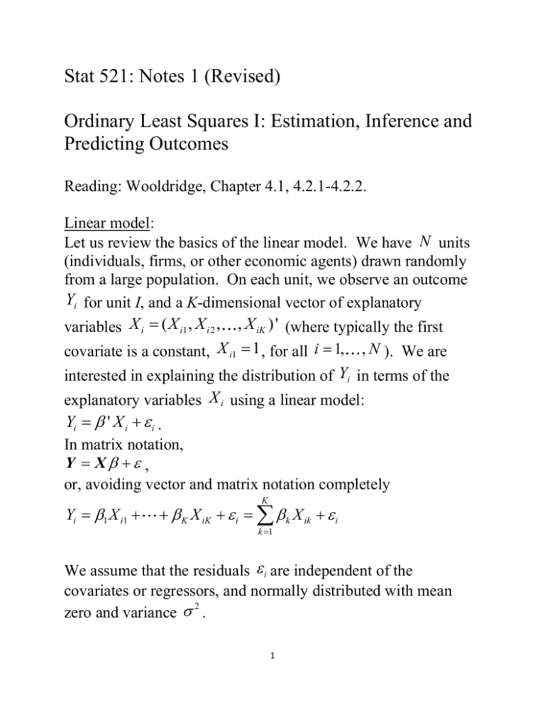
Stat 521: Notes 1 (Revised)
Ordinary Least Squares I: Estimation, Inference and
Predicting Outcomes
Reading: Wooldridge, Chapter 4.1, 4.2.1-4.2.2.
Linear model:
Let us review the basics of the linear model. We have N units
(individuals, firms, or other economic agents) drawn randomly
from a large population. On each unit, we observe an outcome
Yi for unit I, and a K-dimensional vector of explanatory
variables X i  ( X i1 , X i 2 , , X iK ) ' (where typically the first
covariate is a constant, X i1  1 , for all i  1, , N ). We are
interested in explaining the distribution of Yi in terms of the
explanatory variables X i using a linear model:
Yi   ' X i   i .
In matrix notation,
Y  X  ,
or, avoiding vector and matrix notation completely
Yi  1 X i1 
K
  K X iK   i    k X ik   i
k 1
We assume that the residuals  i are independent of the
covariates or regressors, and normally distributed with mean
2
zero and variance  .
1
Assumption 1:  i independent of X i and distributed normally
2
with mean zero and variance  .
The regression model with assumption 1 is called the normal
linear regression model.
We can weaken this considerably. First, we could relax
normality and only assume independence:
Assumption 2:  i independent of X i with mean zero.
We can even weaken this assumption further by requiring only
mean independence
Assumption 3: E ( i | X i )  0 .
Assumption 3 allows for the variance of  i to depend on X i ,
i.e., it allows for heteroskedasticity.
Under Assumptions 1, 2 or 3, we have
E (Yi | X  X i )   ' X i
We will also assume that the observations are drawn randomly
from some population. We can also do most of the analysis by
assuming that the covariates are fixed, but this complicates
matters for some results, and it does not help very much. See
the discussion on fixed versus random covariates in Wooldridge
(page 9).
Assumption 4: The pairs ( X i , Yi ) are independent draws from
some distribution, with the first two moments of X i finite.
The ordinary least squares (OLS) estimator for  solves
2
N
min  (Yi   ' X i ) 2 .

i 1
This leads to
ˆ  ( X ' X ) 1 ( X 'Y )
Under Assumption 1, the exact distribution of the OLS estimator
is
ˆ ~ N   ,  2 ( X ' X ) 1  .
Without assuming that the  i are normally distributed, it is
difficult to derive the exact distribution of ˆ . However, under
the independence Assumption 2 and a second moment condition
2
on  i (variance finite and equal to  ), we can establish
asymptotic normality:
d
N ˆ   
 N (0,  2 E[ X i ' X i ]1 )


Typically, we do not know  . We can consistently estimate it
as
N
2
1
2
ˆ
ˆ
 
 Yi   ' X i
N  K i 1
Dividing by N  K rather than N corrects for the fact that K
parameters are estimated before calculating the residuals
ˆi  Yi  ˆ ' X i . This correction does not matter in large samples,
and in fact the maximum likelihood estimator
2
1 N
2
ˆ
ˆ MLE   Yi   ' X i
N i 1
2




3
is a perfectly reasonable alternative.
In practice, we use the following approximate distribution for ˆ
ˆ  N (  ,Vˆ )
where
V
2
N
 E[ X i ' X i ]
1
  2  E[ X i ' X i ]
1
and
N


2
Vˆ  ˆ   X i X i' 
 i 1

1
Often, we are interested in one particular coefficient. Suppose
for example we are interested in  k . In that case we have
ˆ  N ( ,Vˆ )
k
1
kk
where Vij is the (i, j) element of the matrix V . We can use this
for constructing confidence intervals for a particular coefficient.
A 95% confidence interval for  k is
 ˆ 1.96 Vˆ , ˆ 1.96 Vˆ  .
k
kk
k
kk
We can also use this to test whether a particular coefficient is
equal to some preset number. For example, if we want to test
whether  k is equal to 0.1, we construct the t-statistic
ˆk  0.1
t
Vˆkk
4
Under the null hypothesis that  k is equal to 0.1, t has a
standard normal distribution. We reject the null hypothesis at
the 0.05 level if | t | 1.96 .
Example: Returns to Education
The following regressions are estimated on data from the
National Longitudinal Survey of Youth (NLSY). The data set
used here consists of 935 observations on usual weekly earnings,
years of education, and experience (calculated as age minus
education minus six). The particular data set consists of men
between 28 and 38 years of age at the time wages were
measured.
nlsdata=read.table("nlsdata.txt");
logwage=nlsdata$V1;
educ=nlsdata$V2;
exper=nlsdata$V3;
age=nlsdata$V4;
wage=exp(logwage)
Summary statistics:
> summary(wage);
Min. 1st Qu. Median Mean 3rd Qu. Max.
57.73 288.50 389.10 421.00 500.10 2001.00
> summary(logwage);
Min. 1st Qu. Median Mean 3rd Qu. Max.
4.056 5.665 5.964 5.945 6.215 7.601
> summary(educ);
Min. 1st Qu. Median Mean 3rd Qu. Max.
9.00 12.00 12.00 13.47 16.00 18.00
> summary(exper);
Min. 1st Qu. Median Mean 3rd Qu. Max.
5.00 11.00 13.00 13.62 17.00 23.00
> summary(age);
5
Min. 1st Qu. Median Mean 3rd Qu. Max.
28.00 30.00 33.00 33.09 36.00 38.00
We will use these data to look at returns to education. Mincer
developed a model that leads to the following relation between
log earnings, education and experience for individual i:
log(earnings)i  1   2educi  3experi  3experi 2   i
Estimating this on the NLSY data leads to:
# Returns to education regression
expersq=exper^2;
model1=lm(logwage~educ+exper+expersq);
summary(model1)
Call:
lm(formula = logwage ~ educ + exper + expersq)
Residuals:
Min
1Q Median
3Q Max
-1.70122 -0.25923 0.02022 0.27467 1.68870
Coefficients:
Estimate Std. Error t value Pr(>|t|)
(Intercept) 4.0305512 0.2230182 18.073 <2e-16 ***
educ
0.0925137 0.0075808 12.204 <2e-16 ***
exper
0.0767769 0.0250032 3.071 0.0022 **
expersq -0.0018859 0.0008723 -2.162 0.0309 *
--Signif. codes: 0 ‘***’ 0.001 ‘**’ 0.01 ‘*’ 0.05 ‘.’ 0.1 ‘ ’ 1
Residual standard error: 0.4106 on 926 degrees of freedom
Multiple R-squared: 0.1429, Adjusted R-squared: 0.1401
F-statistic: 51.44 on 3 and 926 DF, p-value: < 2.2e-16
The estimated standard deviation of the residuals is ˆ  0.41 .
6
We will examine more about whether Assumption 1 for the
linear model approximately holds for this data later, but for now
let’s assume that the assumption approximately holds.
Using the estimates and standard errors, we can construct the
confidence intervals. For example, a 95% confidence interval
for the returns to education, measured by the parameter  2 , is
 0.0923 1.96*0.008, 0.0923 1.96*0.008  (0.0775, 0.1071) .
The t-statistic for testing  2  0.1 is
0.0923  0.1
t
 1.0172
0.008
Since | t | 1.96 , at the 0.05 level, we do not reject the hypothesis
that  2 is equal to 0.1.
Now suppose we wish to use these estimates for predicting a
more complex change. For example, suppose we want to see
what the estimated effect is on the log of weekly earnings of
increasing a person’s education by one year. Because changing
an individual’s education also changes their experience (in this
case it automatically reduces it by one year), this effect depends
not just on  2 . To make this specific, let us focus on an
individual with 12 years of education (high school) and ten years
of experience (so that exper2 is equal to 100). The expected
value of this person’s log earnings is
Eˆ (log earnings|educ=12,exper=10)  4.016  0.092*12  0.079*10  0.002*10  5.7191
> # Expected value of log earnings for person with 12 years of education (high
> # school) and ten years of experience
7
>
coef(model1)[1]+coef(model1)[2]*12+coef(model1)[3]*10+coef(model1)[4]*100;
(Intercept)
5.719899
Now change this person’s education to 13. Their experience
will go down to 9 and exper2 down to 81. Hence, their expected
log earnings is
Eˆ (log earnings|educ=13,exper=9)  4.016  0.092 *13  0.079*9  0.002*81  5.7696
> # Expected value of log earnings for person with 13 years of education (high
> # school) and nine years of experience
> coef(model1)[1]+coef(model1)[2]*12+coef(model1)[3]*9+coef(model1)[4]*81;
(Intercept)
5.678954
The difference is ˆ2  ˆ3  19* ˆ4  0.0505 . Hence, the
expected gain of an additional year of education, taking into
account the effect on experience and experience squared is the
difference between these two predictions, which is equal to
0.051. Now the question is what the standard error for this
prediction is. The general way to answer this question is as
follows. The vector of estimated coefficients ˆ is
approximately normal with mean  and variance V . We are
interested in a linear combination of the  ’s, namely
2  3  19* 4   '  where   (0,1, 1, 19) ' . Therefore,
 '  ~ N ( '  ,  ' V  )
1
N
2
'
ˆ
ˆ
V


X
X
  i i  . The command
We estimate V by
 i 1

vcov(model) in R finds Vˆ .
8
> vcov(model1)
(Intercept)
educ
exper
expersq
(Intercept) 0.0497371031 -0.0011370835603 -0.00468369754 0.0001476767044
educ
-0.0011370836 0.0000574686547 0.00003473218 -0.0000005506074
exper
-0.0046836975 0.0000347321798 0.00062516139 -0.0000214799425
expersq 0.0001476767 -0.0000005506074 -0.00002147994 0.0000007609628
> # Standard error and confidence interval for effect on expected log earnings
> # of increasing education by 1 when education starts at 12 and experience
> # starts at ten
> lambda=matrix(c(0,1,-1,-19),ncol=1);
> betahat=matrix(coef(model1),ncol=1);
> estimate=t(lambda)%*%betahat;
> var.est=t(lambda)%*%vcov(model1)%*%lambda;
> se.est=sqrt(var.est);
> lci=estimate-1.96*se.est;
> uci=estimate+1.96*se.est;
> estimate
[,1]
[1,] 0.05156802
> se.est
[,1]
[1,] 0.009620735
> lci
[,1]
[1,] 0.03271138
> uci
[,1]
[1,] 0.07042466
Thus, the 95% confidence for the change in expected log
earnings from the one year increase in education, when eduation
started at 12 and experience at ten, is (0.0327, 0.0704).
The Delta Method
9
The above method works for finding the standard error of a
linear function of the coefficients in the regression model. The
delta method is a method for finding the standard error of a
nonlinear function of the coefficients.
Example: Suppose we just consider the regression of log
earnings on education.
> model2=lm(logwage~educ);
> summary(model2);
Call:
lm(formula = logwage ~ educ)
Residuals:
Min
1Q Median
3Q Max
-1.79050 -0.25453 0.01991 0.27309 1.68779
Coefficients:
Estimate Std. Error t value Pr(>|t|)
(Intercept) 5.040344 0.085044 59.27 <2e-16 ***
educ
0.067168 0.006231 10.78 <2e-16 ***
--Signif. codes: 0 ‘***’ 0.001 ‘**’ 0.01 ‘*’ 0.05 ‘.’ 0.1 ‘ ’ 1
Residual standard error: 0.4177 on 928 degrees of freedom
Multiple R-squared: 0.1113, Adjusted R-squared: 0.1103
F-statistic: 116.2 on 1 and 928 DF, p-value: < 2.2e-16
The estimated regression function is
E (log earnings | educ  x)  5.0403  0.0672* x
2
2
The estimate for  is ˆ  0.4177  0.1744 . Let’s assume
Assumption 1 holds (we will examine more later).
2
10
Suppose we are interested in the average effect of increasing
education by one year for an individual with currently eight
years of education, not on the log of earnings, but on the level of
earnings.
2
Then, using the fact that if Z ~ N (  ,  ) , then
E[exp( Z )]  exp(    2 / 2) , we have
E (earnings | educ  x)  exp( 1   2 * x   2 / 2) .
Hence, the parameter of interest (the effect of increasing
education from eight to nine) is
  exp( 1   2 *9   2 / 2)  exp( 1   2 *8   2 / 2)
Getting an estimate for  is easy. Just plug in the estimates for
 and  2 to get
ˆ  exp(ˆ1  ˆ2 *9  ˆ 2 / 2)  exp(ˆ1  ˆ2 *8  ˆ 2 / 2)  20.0480 .
> # Estimated effect of increasing education from eight to nine on earnings
sigmahatsq=.4177^2;
thetahat=exp(coef(model2)[1]+coef(model2)[2]*9+sigmahatsq/2)exp(coef(model2)[1]+coef(model2)[2]*8+sigmahatsq/2);
> thetahat
(Intercept)
20.04802
However, we also need a standard error for this estimate. Let us
write the parameter of interest more generally as   g ( )
2
where   (  ',  ) ' .
Delta Method: Suppose that for some estimate ˆ of a true
parameter  , we have N (ˆ   )  N (0, ) . Then,
11
 g
g 
N  g (ˆ )  g ( )   N  0, '   .
 
 
Another way of stating the Delta method is the following:



ˆ




N
(0,

)
Suppose
where
N . Then
 g g 
( g (ˆ )  g ( ))  N  0, '   .
 
 
In our case,
g ( )  exp( 1   2 *9   2 / 2)  exp( 1   2 *8   2 / 2)
and


2
2
 exp( 1   2 *9   / 2)  exp( 1   2 *8   / 2)


g 
  9*exp( 1   2 *9   2 / 2)  8*exp( 1   2 *8   2 / 2) 
 

1
2
2
 exp( 1   2 *9   / 2)  8*exp( 1   2 *8   / 2) 
2

We estimate this by substituting estimated values for the
parameters, so we get


2
2
ˆ
ˆ
ˆ
ˆ
ˆ
ˆ
 exp( 1   2 *9   / 2)  exp( 1   2 *8   / 2)


g 
  9*exp( ˆ1  ˆ2 *9  ˆ 2 / 2)  8*exp( ˆ1  ˆ2 *8  ˆ 2 / 2) 
 

1
1
2
2
ˆ
ˆ
ˆ
ˆ
 exp( 1   2 *9  ˆ / 2)  *exp( 1   2 *8  ˆ / 2) 
2
2

partialg.partialgamma.1=exp(coef(model2)[1]+coef(model2)[2]*9+sigmahatsq/2)exp(coef(model2)[1]+coef(model2)[2]*8+sigmahatsq/2);
12
partialg.partialgamma.2=9*exp(coef(model2)[1]+coef(model2)[2]*9+sigmahatsq/2
)-8*exp(coef(model2)[1]+coef(model2)[2]*8+sigmahatsq/2);
partialg.partialgamma.3=.5*exp(coef(model2)[1]+coef(model2)[2]*9+sigmahatsq/
2)-.5*exp(coef(model2)[1]+coef(model2)[2]*8+sigmahatsq/2);
> partialg.partialgamma.1
(Intercept)
20.04802
> partialg.partialgamma.2
(Intercept)
468.9977
> partialg.partialgamma.3
(Intercept)
10.02401
To get the variance  for ˆ  g (ˆ ) , we also need the full
2
covariance matrix of   ( 1 ,  2 ,  ) ' . We have the following
distributional fact for the normal linear regression model:
N
2
Under the normal linear regression model, ˆ 
is independent of ˆ and
( N  K )ˆ 2
2
 (Y  ˆ ' X )
i 1
i
N K
~  N2  K (Searle, Linear
2
Models, Chapter 5.3). The variance of a  m (chi-squared
distribution with m degrees of freedom) is 2m . Thus,
4
2 4
2
Var (ˆ ) 
2( N  K ) 
2
(N  K )
N  K and we can estimate
4
ˆ
2

Var (ˆ 2 ) by
N K .
2*0.17444
ˆ (ˆ ) 
 0.000066 .
Hence we have Var
930  2
2
13
i
2
We also have
> vcov(model2);
(Intercept)
educ
(Intercept) 0.0072324477 -0.00052296635
educ
-0.0005229664 0.00003882174
so
v=vcov(model2);
Lambdahat=matrix(c(v[1,1],v[2,1],0,v[1,2],v[2,2],0,0,0,.000066),ncol=3);
> Lambdahat
[,1]
[,2] [,3]
[1,] 0.0072324477 -5.229664e-04 0.0e+00
[2,] -0.0005229664 3.882174e-05 0.0e+00
[3,] 0.0000000000 0.000000e+00 6.6e-05
and the variance for ˆ is
g
ˆ g (ˆ )
(ˆ ) ' 


partialg.partialgamma=matrix(c(partialg.partialgamma.1,partialg.partialgamma.2,p
artialg.partialgamma.3),ncol=1);
varthetahat=t(partialg.partialgamma)%*%Lambdahat%*%partialg.partialgamma;
> varthetahat
[,1]
[1,] 1.618347
Hence, a 95% confidence interval for  (the effect on expected
earnings of increasing education from 8 to 9) is
lci.theta=thetahat-1.96*sqrt(varthetahat);
uci.theta=thetahat+1.96*sqrt(varthetahat);
> lci.theta
[,1]
[1,] 17.55462
> uci.theta
[,1]
[1,] 22.54142
14