Mathematical modeling:
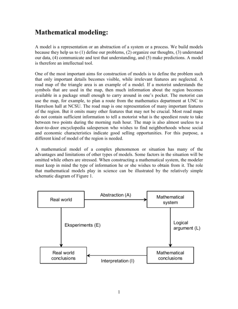
A model is a representation or an abstraction of a system or a process. We build models
because they help us to (1) define our problems, (2) organize our thoughts, (3) understand
our data, (4) communicate and test that understanding, and (5) make predictions. A model
is therefore an intellectual tool.
One of the most important aims for construction of models is to define the problem such
that only important details becomes visible, while irrelevant features are neglected. A
road map of the triangle area is an example of a model. If a motorist understands the
symbols that are used in the map, then much information about the region becomes
available in a package small enough to carry around in one’s pocket. The motorist can
use the map, for example, to plan a route from the mathematics department at UNC to
Harrelson hall at NCSU. The road map is one representation of many important features
of the region. But it omits many other features that may not be crucial. Most road maps
do not contain sufficient information to tell a motorist what is the speediest route to take
between two points during the morning rush hour. The map is also almost useless to a
door-to-door encyclopedia salesperson who wishes to find neighborhoods whose social
and economic characteristics indicate good selling opportunities. For this purpose, a
different kind of model of the region is needed.
A mathematical model of a complex phenomenon or situation has many of the
advantages and limitations of other types of models. Some factors in the situation will be
omitted while others are stressed. When constructing a mathematical system, the modeler
must keep in mind the type of information he or she wishes to obtain from it. The role
that mathematical models play in science can be illustrated by the relatively simple
schematic diagram of Figure 1.
Abstraction (A)
Real world
Logical
argument (L)
Eksperiments (E)
Real world
conclusions
Mathematical
system
Interpretation (I)
1
Mathematical
conclusions
The scientist begins with some observations about the real world. He or she wishes to
make some conclusions or predictions about the situation he or she has observed. One
way to proceed (E) is to conduct some experiments and record the results. The model
builder follows a different path. First, he or she abstracts, or translates, some of the
essential features of the real world into a mathematical system. Then by logical argument
(L) he or she derives some mathematical conclusions. These conclusions are then
interpreted (I) as predictions about the real world. To be useful, the mathematical system
should predict conclusions about the real world that are actually observed when
appropriate experiments are carried out. If the predictions from the model bear little
resemblance to what actually occurs in the real world, then the model is not a good one.
The modeler has not isolated the critical features of the situation being studied or the
axioms misrepresent the relations among these features. On the other hand, if there is
good agreement between what is observed and what the model predicts, then there is
some reason to believe that the mathematical system does indeed capture correctly
important aspects of the real-world situation.
What happens quite frequently is that some of the predictions of a mathematical model
agree quite closely with observed events, while other predictions do not agree with the
observed events. In such a case, we might hope to modify the model to improve its
accuracy. The incorrect predictions may suggest ways of rethinking the assumptions of
the mathematical system. One hopes that the revised model will not only preserve the
correct predictions of the original one, but that it will also make further correct
predictions. The incorrect inferences of the revised model will lead, in turn, to yet another
version, more sophisticated more accurate than the previous one.
However, it is important to keep in mind, that the goal is not to make the most precise
model of the part of the world that is modeled, but that the model (like the road map)
includes all the essential features, even if that means that some other features in the
model do not present the reality. For example, a model of the cardiovascular system (the
heart, arteries, and veins) could accurately present the systemic arteries and veins and
then lump the pulmonary circulation into a single compartment. Such a compartment
would never represent any of the subsystems correctly.
When building mathematical models one should distinguish between the different types
of models, some models (deterministic models) can be derived directly from physical
laws (e.g. Newton’s second law), while other models are based on empirical
observations. Both types of models provide insight into the system modeled, but the type
of model must be considered carefully. For example, very different types of models are
used for predict the weather tomorrow and to determine a rockets trajectory to the moon.
Holling (1978) has a diagram (Figure 2) that provides a simple and useful classification
of problems. The horizontal axis represents how well we understand the problem we are
trying to solve; the vertical axis represents the quality and/or quantity of relevant data
(Figure 2). Holling divides the quadrant between the two axes into four areas,
corresponding to four classes of problems.
2
3
4
2
Data
1
Understanding
Area 1 is a region with good data but little understanding. This is where statistical
techniques are useful; they enable one to analyze the data search for patterns or relation,
construct and test hypotheses, and so on.
Area 3 is a region with good data and good understanding. Many problems in engineering
and the physical sciences (for example, the problem of computing a rockets trajectory to
the moon) belong to this class of problems. This is the area where models are used
routinely and with confidence because their effectiveness has been proved repeatedly.
Area 2 has little in the way of supporting data but there is some understanding of the
structure of the problem.
Area 4, in this area there is little knowledge of the structure of the problem and little data
to support it.
Unfortunately, many problems in the nonphysical sciences (especially in the biological
sciences) belong to areas 2 and 4. However, recent explosion in experimental techniques
move some of these problems to areas 1 and 3. The main difference from the physical
problems is the uncertainty and high levels of noise often found in the data.
The modeling challenges for problems in area 2 and 4 are:
-
Decisions may have to be made despite the lack of data and understanding.
How do we make good, scientific decision under these circumstances?
How do we go about improving our understanding and suggest new ways for
collecting the data necessary to validate the modeling. This is an area where
modeling can be used to predict new experimental settings.
3
Models that lie in areas 2 and 4 are bound to be speculative. They will never have the
respectability of models build for solving problems in area 3 because it is unlikely they
will be sufficiently accurate of that they can ever be tested conclusively. In fact most
models in biology cannot be tested conclusively, while we have a lot more data today that
20 years ago there are still many types of data that could validate models, but that are
unethical to measure. Models build this way should never be used unquestioningly or
automatically. The whole process of building and using these models has to be that much
more thoughtful because we do not really understand the structure of the problem and do
not have (and cannot easily get) supporting data.
We therefore build models to explore the consequences of what we believe to be true.
Those who have a lot of data and little understanding of their problem (area 1) gain
understanding by “living with” their data, looking at it in different ways, and searching
for patterns and relationships. Because we have so little data in areas 2 and 4, we learn
by living with our models, by exercising them, manipulating them, questioning their
relevance, and comparing their behavior with what we know (or think we know) about
the real world. This process often forces us to reevaluate our beliefs, and that reevaluation
in turn leads to new versions off the models. The mere act of assembling the pieces and
building a model (however speculative the model might be) usually improves our
understanding and enables us to find or use data we had not realized were relevant. That
in turn leads us to a better model.
The process is one of boot-strapping: If we begin with little data and understanding in the
bottom left-hand corner of Holling’s diagram, models help us to zigzag upwards and to
the right. This is a far healthier approach than one of just collecting data because we
improve our understanding as we go along. (Those who collect data without building
models run the very real risk of discovering, when they eventually analyze their data, that
they have collected the wrong data!)
4
The modeling process:
The real world
(a) problem formulation
Part of the real world
(the problem)
(b) System identification
System
(c) Mathematical formulation
Mathematical system
(d) Mathematical analysis
Model results
(e) Interpretation and analysis of results
Action/Insight
(f) Analysis of the model validity
References:
“BASE Note 1”, Morten Blomhoj, Tinne Hoff Kjeldsen, Johnny Ottesen, Natural
Sciences Basis Program, Roskilde University Center, Denmark, August 2000.
“An Introduction to Mathematical Models in the Social and Life Sciences”, Michael
Olinick, Addison-Wesley Publishing Company, Massachusetts, 1978.
“Building Models for Conservation and Wildlife Management”, Second edition, A.M.
Starfield, A.L. Bleloch, Burgess International Group Inc., Minnesota, 1991.
5