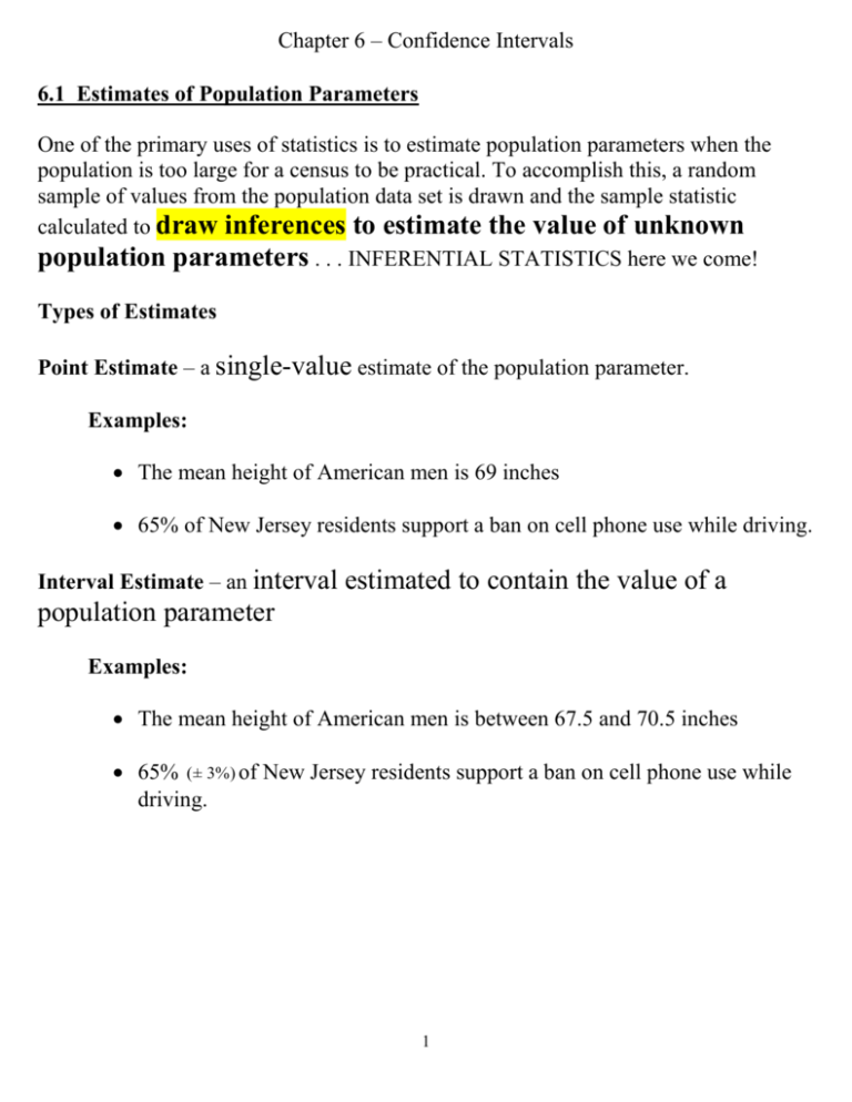
Chapter 6 – Confidence Intervals
6.1 Estimates of Population Parameters
One of the primary uses of statistics is to estimate population parameters when the
population is too large for a census to be practical. To accomplish this, a random
sample of values from the population data set is drawn and the sample statistic
calculated to draw inferences to estimate the value of unknown
population parameters . . . INFERENTIAL STATISTICS here we come!
Types of Estimates
Point Estimate – a single-value estimate of the population parameter.
Examples:
 The mean height of American men is 69 inches
 65% of New Jersey residents support a ban on cell phone use while driving.
Interval Estimate – an interval
estimated to contain the value of a
population parameter
Examples:
 The mean height of American men is between 67.5 and 70.5 inches
 65% (± 3%) of New Jersey residents support a ban on cell phone use while
driving.
1
Level of Confidence
A point estimate is almost sure to differ from the actual population parameter (at least
slightly), while a good interval estimate can be quite likely to contain the population
parameter.
The level of confidence for an interval estimate is the probability that the
interval contains the population parameter. The level of confidence is
denoted by c, the area under the standard normal curve between the critical
values of –zc and zc. The most commonly used values of c are .90, .95, and .99.
Examples:
 The mean height of American men is between 67.5 and 70.5 inches with a level
of confidence of c  .90
 With 95% confidence, we can say that 65% (± 3%) of New Jersey residents
support a ban on cell phone use while driving.
Note: The level of confidence is a probability for the experiment of drawing a sample
and constructing an interval estimate. That is, though there will be a natural variation
between samples, c is the percent of these sample means that will be between –zc and
zc.
The first example above can be interpreted as follows:
Whenever a sample of American men is drawn and an interval estimate is
constructed from the sample data, 90% of the samples will yield an interval
estimate that contains the actual mean height of all men. Another way of wording
this is that we are 90% sure (confident) that the true (population) mean height of
all American men is within this interval.
2
Estimating the Mean
Point Estimate – If we wish to estimate the population mean  for a random
variable x using a sample of values, the best possible point estimate is just
the sample mean x .
Interval Estimate – We construct an interval estimate for  by starting with the
sample mean x and adding a margin of error denoted by E both above
and below x . We will then have an interval estimate of the form:
( x  E, x  E )
Example: For the estimate of men’s heights given above, the sample average x was
69 inches and a margin of error of E  1.5 inches was used to get the interval estimate
( x  E , x  E )  (69  1.5, 69  1.5)  (67.5, 70.5)
Note: The margin
of error used for an interval estimate depends
on the level of confidence desired. A larger level of confidence will result in
a _______________ margin of error, and hence a _______________ interval.
Usually, the level of confidence is selected, and then the corresponding margin of error
necessary is calculated.
3
Calculating Margin of Error with a Large Sample
If the random variable x is normally distributed (with a known standard
deviation  ) or if the sample size n is at least 30, then since we will be drawing a
random sample and taking the sample mean x , we can apply the Central
Limit Theorem. In this case, The Central Limit Theorem guarantees us that:
 x is approximately normally distributed
 x  
 x  n
Notice that the mean value of x is equal to  the population mean we are trying to
estimate. Given the desired level of confidence c, we are now trying to find the
amount of error E necessary to ensure that the probability of x being within E of the
mean is c.
There are always two critical z-scores  zc which give the appropriate probability for
the standard normal distribution (see diagram in book p. 282), and so the
corresponding probability for the distribution of x is just zc   x or:
E  zc

n
Note: Usually  is not known, but if n  30 , then the sample standard deviation s is
generally a reasonable estimate.
Before continuing, lest practice finding zc for a confidence level of:
c = 0.90
c = 0.95
c = 0.97
4
Example: Suppose a random sample of 40 American men is drawn and the weights of
the men measured. If the sample mean is x  182 lbs. and sample standard deviation is
s  18.4 lbs., then we can construct a 90% confidence interval for the mean weight of the
population of American men as follows.
Since
c  .90
we look up the value
1 c
 .05
2
in the standard normal table and find that it
corresponds to a z-score of z  1.645 thus we will use 1.645 for
error can now be calculated using the formula:

18.4
E  zc
n
 (1.645) 
40
zc .
The margin of
 4.8
Therefore, based on our sample data we are 90% confident that the average weight of
all American men is within 4.8 lbs. of our sample average. From this we get that our
90% confidence interval is: ( x  E , x  E )  (182  4.8,182  4.8)  (177.2,186.8)
Exercise: Construct a 95% confidence interval from the above data.
5
Example: A survey of 100 Tampa commuters finds that the average commuting time
to work is x  25.5 minutes with a standard deviation of s  11.5 minutes. We can
construct a 98% confidence interval for the mean commuting time of Tampa
commuters as follows.
Since
c  .98
we look up the value
in the standard normal table
and find that it corresponds to a z-score of
thus we will use
for
zc .
The margin of error can now be calculated using the formula:
E  zc 
n
And our 98% confidence interval is:
( x  E, x  E )=
So based on our sample data, we can be 98% sure that the average commuting time of
Tampa commuters is between
and
minutes.
Exercise: Repeat the above, but suppose the sample size had been only 50
commuters. What happens to the margin of error? (Make a guess, now see if you were
right by computing the interval.)
6
Example: From previous examples we know that the heights of American women
ages 20-29 are normally distributed with a standard deviation of   2.75 inches.
If we did not know the mean height of all women, we could use the following sample
of 5 women’s heights to estimate  :
67, 63, 64, 65, 63
The sample average is x  64.4 inches for this sample. We can now construct a 95%
confidence interval for  . Since a probability of .025 corresponds to a z-score of
z  1.96 , we will use 1.96 for zc . We again use the formula:

2.75
E  zc
n
 (1.96) 
5
 2.4
to get a margin of error of 2.4 inches. The corresponding 95% confidence interval is:
( x  E , x  E )  (64.4  2.4, 64.4  2.4)  (62, 66.8)
So based on our sample we are 95% confident that 62    66.8 . Note that this interval
contains the previously given value   63.5 . If many samples of 5 women were drawn,
95% of the sample means would be within 2.4 inches of 63.5.
Determining Sample Size
Note: Given a confidence level c, and standard deviation  , drawing a larger sample
will _______crease the margin of error.
If a desired margin of error and level of confidence are known, and if an estimate of
the standard deviation can be made, then the sample size necessary can be determined
by solving the error formula for n.
We know:
E  zc
multiplying by
n

n
yields:
E n  zc
dividing by E we obtain:
n
zc
E
z 
n   c  Always round UP!
 E 
2
finally, squaring both sides yields:
7
Example: Suppose we want to estimate the mean weight of American men, and we
want to be 95% confident that our estimate is within 2 lbs. of the actual mean. Since
our previous study allows us to estimate that the standard deviation of men’s weights
is   18.4 pounds, we can use the formula above to determine the appropriate sample
size.
From the given information, we have c  .95 , so zc  1.96 , the maximum desired error
is E  2 , and we estimated that   18.4 , so:
 z    1.96 18.4 
n c  
  325.15
2

 E  
2
2
Thus a sample of ___________ men should give the desired level of accuracy.
Exercise: Calculate the number of Tampa commuters it would be necessary to
measure the commute for in order to estimate the mean commuting time to within 1
minute with 99% confidence. (From a previous example we had: a survey of 100
Tampa commuters finds that the average commuting time to work is x  25.5 minutes
with a standard deviation of s  11.5 minutes.)
Do page 320 # 56 together to be turned in. Now let’s sample our class and use the data
we have to construct a 90% confidence interval for the average age of a college
student. What had to change for us to do this with a smaller sample than required?
How might sampling just our class be a confounding issue?
8
6.2
The (Student) t-distributions
In the last example we were able to construct a confidence interval with a small
sample ( n  5 ) because the variable women’s heights is normally distributed.
Unfortunately, it was necessary that we knew the population standard deviation  .
is very unlikely in any real-life situation that we would know 
yet be trying to estimate  .
It
and
A good solution would be to use the sample standard deviation s from our small
sample to estimate  , but the estimation of  from a small sample is generally not
accurate enough for use in the normal distribution test.
If x is normally distributed, then the distribution of
z
x 
/ n
is the standard normal distribution for any sample size n, but the distribution of
t
x 
s/ n
is not. The distribution of the random variable above is the Student t-distribution
with n – 1degrees of freedom (d.f.).
Properties of t-distributions
The t-distributions are a family of probability density functions. For each possible
degree of freedom, there is a unique t-distribution with that degree of freedom.
Like the standard normal distribution, the t-distributions are symmetric, bell-shaped
probability density functions with a mean of 0. However, the t-distribution is
a
wider bell curve with thicker tails than the standard normal
curve.
As the degree of freedom increases, the t-distributions become closer to a normal
distribution. Thus for large sample sizes ( n  30 ), we can use s in place of  , and then
use the standard normal distribution.
See diagram and box on page 325 of the text. SEE PAGE 329 FLOW CHART!
9
Estimating the Mean Using a t-distribution
The process of constructing a confidence interval using a t-distribution is almost
identical to that used to construct confidence intervals using the standard normal
distribution.
First we must know that the variable x is normally
distributed with
unknown standard deviation σ and that we will draw a small
sample (n < 30).
We then choose c, the desired level of confidence, and calculate the statistics x and s
from our sample group.
The sample mean x will again be the best point estimate and the center of our interval.
We can then calculate the margin of error for our estimate using the formula:
E  tc
s
n
Where tc is the critical t-value corresponding to the level of confidence c. The values
of tc for common values of c are given in a table in the front of your text.
sure to use a degree of freedom of
n 1
Make
.
Note: tc  zc for the same value of c since the t-distribution is wider, so we get a
larger margin of error using the t-distribution.
10
Example: Suppose we had our sample of 5 women’s heights from the previous
example:
67, 63, 64, 65, 63
If we knew that women’s heights were normally distributed, but did not know that
  2.75 inches, then we would use the sample standard deviation s as our estimate of  ,
and then use a t-distribution interval.
The sample mean is
x  64.4 inches
and the sample standard deviation is s  1.67 inches.
For 95% confidence, the critical t-score for degree of freedom _____ is:
So:
E  tc
s
 1.67 
 (2.776) 
  2.07
n
 5 
and so our 95% confidence interval is: (64.4  2.07, 64.4  2.07)  (62.33, 66.47)
Exercise: Construct a 99% confidence interval from the above data.
11
tc  2.776
Example: SAT Math Scores are normally distributed. A sample of scores for 20
students has sample mean of x  522.8 with a sample standard deviation of s  154.5 .
We can calculate the 90% confidence interval as follows:
For 90% confidence, the critical t-score for degree of freedom 19 is:
So:
E  tc
tc  1.729
s
 154.5 
 (1.729) 
  59.7
n
20


and our 90% confidence interval is: (522.8  59.7,522.8  59.7)  (463.1,582.5)
Exercises:
 Suppose the same sample mean and sample standard deviation had been obtained
from a sample of size 16. What would the 90% confidence interval be?
 Suppose the same sample mean and sample standard deviation were obtained
from a sample of size 50. What would the 90% confidence interval be?
If time: p 332 # 30. Be sure to do #29 for homework.
12
6.3 Estimating a Population Proportion
Often, we wish to estimate what portion or percentage of a population falls into a
given category.
Examples: (What type of data is being measured here: qualitative or
quantitative?
 What percent of Florida voters plan to vote for the Democratic candidate for
senate?
 What percent of people have Type A+ blood?
 What percent of computer processors are defective?
Such a percentage is called a population proportion and is represented by the
variable p, (the probability of success in a single trial of a binomial experiment). The
proportion calculated in a sample group is denoted by p̂ (“p hat”) and is the best
point estimate for p. If we have a sample of size n where x of the sample members
are in the category being measured, then we calculate
p̂
(proportion
of sample’s successes) by using:
ˆ 
p
x
n
Where x = the number of successes in the sample, and n = the number in the sample.
Example: In a sample of 577 computer processors, 37 were found to be defective.
Thus if p̂ represents the proportion of defective processors, then:
pˆ 
x 37

 .064
n 577
So we might estimate that 6.4% of processors are defective.
13
The Sampling Distribution of
p̂
We construct interval estimates for p in much the same way as our confidence
intervals for a mean. We can calculate p̂ and use it as the center of
our
interval and then add a margin of error above and below p̂ .
The experiment of drawing a sample of n objects and counting the number x in the
desired category is a binomial experiment with n trials and probability of success p on
each trial (as long as the population is very large compared to n). If a sample is
sufficiently large however, then the average number of successes p̂ will be
approximately normally distributed. More specifically:
If an n trial binomial experiment is conducted with probability of success p, and if
np > 5 and nq > 5, then the distribution of the random variable p̂ is
approximately normal with:
 pˆ  E ( x / n) 
 pˆ   ( x / n) 
E ( x) np

p
n
n
and
 ( x)
n
14

npq

n
pq
n
Constructing Confidence Intervals for p
From the above we see that we can use the normal distribution to construct confidence
intervals for p. As before, we first decide the desired level of confidence c, and
then find the critical z-score zc . The margin of error is then found by a similar formula
as before:
E  zc pˆ  zc
pq
n
Note: p is the quantity we are trying to estimate, so it is actually unknown, but once
the sample is drawn, we can use p̂ as our estimate for p and qˆ  1  pˆ as our estimate for
q. So in practice, the formula for margin of error in a population proportion estimate
ˆˆ
pq
E

z
c
is:
n
Example: In a study of a microchip manufacturer, 37 out of a sample of 577
processors were found to have defects. We can construct a 95% confidence interval
for the percentage of defective processors as follows:
First we calculate
x
pˆ  
n
, and so
q̂ 
.
Next check that npˆ  x  37  5 and nqˆ  n  x  540  5 . Which means?
Now since c  .95 , we have zc  .
Our margin of error is thus:
ˆˆ
pq
E  zc

n
Our 95% confidence interval is:
( pˆ  E , pˆ  E )  (0.064 -
, 0.064 +
)=(
,
)
So we are 95% confident that the percentage of defective processors is between
and
%.
Exercise: Calculate the 99% confidence interval for this example.
15
%
Example: A new drug is tested on a sample of 75 adults who were infected with a
cold virus. 32% of the adults in the sample developed no symptoms. Construct a 90%
confidence interval for the proportion of adults who will be prevented from getting a
cold by the drug.
From the above we have that n =
,
p̂ =
and
q̂ =
How can we determine if we can approximate the sampling distribution of
the normal distribution?
Find zc: we use the fact that c  .90 to find zc =
Calculate the margin of error E:
E  zc
p̂ using
.
ˆˆ
pq

n
And our 90% confidence interval is:
( pˆ  E , pˆ  E ) 
So with 90% confidence, we can say that between
will be helped by the drug.
% and
% of adults
Exercise: Suppose that the drug company runs a larger study with a sample of 425
adults, and again 32% develop no symptoms. Construct a 98% confidence interval in
this case.
16
Determining Sample Size
As with our estimates of the mean, we often wish to estimate the size of sample
necessary to achieve a certain margin of error and level of confidence.
To determine a formula, we again solve our margin of error formula for n.
We know:
E  zc
multiplying by
n
pq
n
yields:
E n  zc pq
dividing by E we obtain:
n
zc pq
E
finally, squaring both sides yields:
zc2 pq
n 2
E
Notice that this formula depends on our knowing p and q in advance. If estimates are
known, then they may be used, otherwise, we use the fact that since 0  p  1 ,
pq  p(1  p)  .25
Example: Suppose we want to estimate the percent of processors that are defective to
within 1% with 95% confidence. We can determine the necessary sample size as
follows.
If we have no prior estimate of p and q, then we use pq  .25 , and we have the desired
margin of error is E  .01, and since c  .95 , zc  1.96 . So the required sample size is:
zc2 pq (1.96)2 (.25)
n 2 
 9604
E
(.01)2
So a sample of 9604 processors is necessary to obtain the desired accuracy.
Exercise: Repeat the above, but use the fact that our previous study showed
that p  .064 .
17
Using the TI-83 to Construct Confidence Intervals
The TI-83 can make the margin of error and confidence interval calculation given the
level of confidence c, the standard deviation  , sample size n, and sample mean x .
To start the program ZInterval, do the following:
Press [STAT]
Use the arrow keys to highlight the TESTS Menu
Highlight 7: ZInterval from the list and press [ENTER]
A menu now appears on the screen. You can use the down and up arrows to highlight
different entries.
If you know n,  , and x , then make sure Inpt: is set to Stats. If you want the TI-83 to
calculate from a data set, you would choose Data for Inpt:
Enter the values of  , x , n, and c.
When you are finished highlight the word Calculate and press [ENTER]. The
confidence interval will then be calculated and appear on your screen along with
n.
Example: Using the data from our first example:   18.4
x  182 , n  40 , and c  .90 , the ZInterval program gives:
confidence interval.
18
(177.21,186.79) as
the
x
and
Using the TI-83 to Construct t-distribution Intervals
The TI-83 can be used to construct confidence intervals for the t-distributions. Again,
the level of confidence c, the standard deviation  , the sample size n, and the sample
mean x are required.
To start the program TInterval, do the following:
Press [STAT]
Use the arrow keys to highlight the TESTS Menu
Highlight 8: TInterval from the list and press [ENTER]
A menu now appears on the screen. You can use the down and up arrows to highlight
different entries.
As before, if n,  , and x are known, then set Inpt: to Stats, and if using a data set stored
in a list set Inpt: to Data.
Enter the values of  , x , n, and c.
When you are finished highlight the word Calculate and press [ENTER]. The
confidence interval will then be calculated and appear on your screen along with
n.
Example: Using the data from our SAT example:   154.5 , x  522.8 ,
the TInterval program gives: (463.06,582.54) as the confidence interval.
19
n  20 ,
x
and
and c  .90 ,
Using the TI-83 to Construct Population Proportion Confidence Intervals
The TI-83 can be used to construct confidence intervals for population proportions.
The level of confidence c, the sample size n, and the number in the category from the
sample x are required.
To start the program 1-PropZInt, do the following:
Press [STAT]
Use the arrow keys to highlight the TESTS Menu
Highlight A: 1-PropZInt from the list and press [ENTER]
A menu now appears on the screen. You can use the down and up arrows to highlight
different entries.
Enter the values of x, n, and c.
If the value of p̂ is known but not x, then calculate x from the formula x  npˆ .
When you are finished highlight the word Calculate and press [ENTER]. The
confidence interval will then be calculated and appear on your screen along with p̂
and n.
Example: Using the data from our first example: x  37 , n  577 , and c  .95 , the
1-PropZInt program gives: (.04414,.08411) as the confidence interval.
20