Categorical Data Analysis
A. Independence
B. Homogeniety
C. McNemar’s Test -- Analysis from paired designs
D. Cochran Mantel Haenszel Test
E. Mantel-Haenszel Test of Trend
A. Independence
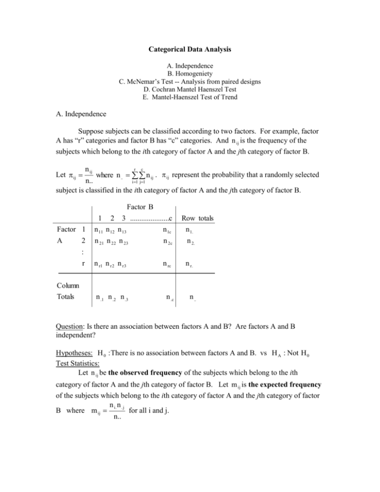
Suppose subjects can be classified according to two factors. For example, factor
A has “r” categories and factor B has “c” categories. And n ij is the frequency of the
subjects which belong to the ith category of factor A and the jth category of factor B.
Let  ij 
n ij
r
c
where n ..   n ij .  ij represent the probability that a randomly selected
n..
i 1 j1
subject is classified in the ith category of factor A and the jth category of factor B.
Factor B
1
2
3 .....................c
Row totals
Factor 1
n 11 n 12 n 13
n 1c
n 1.
A
n 21 n 22 n 23
n 2c
n 2.
n r1 n r 2 n r 3
n rc
n r.
2
:
r
Column
Totals
n .1 n .2 n .3
n .c
n ..
Question: Is there an association between factors A and B? Are factors A and B
independent?
Hypotheses: H 0 : There is no association between factors A and B. vs H A : Not H 0
Test Statistics:
Let n ij be the observed frequency of the subjects which belong to the ith
category of factor A and the jth category of factor B. Let m ij is the expected frequency
of the subjects which belong to the ith category of factor A and the jth category of factor
n i. n . j
B where m ij 
for all i and j.
n..
1) Statistics for testing H o (Pearson’s Chi-Square) is
r
c
  
2
(n ij  m ij ) 2
i 1 j1
m ij
~  2 df ( r 1)( c1)
Reject H 0 if  2   2 .05,( r 1)( c 1) .
2) Likelihood ratio statistic (due to R.A. Fisher; for large sample sizes)
r c
 n ij 
 ~  2 df ( r 1)( c1)
G 2  2  n ij ln 


m
i 1 j1
 ij 
Reject H 0 if G 2   2 .05,( r 1)( c 1) .
Generally,  2 and G 2 are similar.
Note: for both statistics, each expected cell size should be greater than or equal to 5.
m ij  5 . Otherwise, use Fisher’s exact test (2 by 2 table) and generalization (r by
c table).
Example
Is there any association of oral contraceptive use with likelihood of heart attacks?
H 0 : There is no association between two factors vs H A : Not
Factor B
Heart Attacks
Factor A
Yes
No
Oral
Used
23
34
Contraceptive Never Used
35
132
Column Totals
58
166
57 * 58
57 * 166
m11 
 14.76
m12 
 42.24
224
224
167 * 58
167 * 166
m 21 
 43.24
m 22 
 123.76
224
224
H0
Row Totals
57
167
224
(23  14.76) 2 (34  42.24) 2 (35  43.24) 2 (132  123.76) 2



14.76
42.24
43.24
123.76
 8.33
2 
From Table A-3  2 .05,1  3.841 . Reject H 0 since 8.33 > 3.841
Therefore, there is an association between oral contraceptive use with the likelihood of
heart attacks.
B. Homogeneity
Factor B
1
2
3 .....................c
Row totals
Factor 1
n 11 n 12 n 13
n 1c
c1
A
n 21 n 22 n 23
n 2c
c2
n r1 n r 2 n r 3
n rc
cr
2
:
r
Column
Totals
n .1 n .2 n .3
n .c
n ..
Notice that the row totals are a fixed constant in advance.
Conditional probability  ij  Pr{B  j | A  i} =
n ij
ci
Hypotheses
H 0 : There is row homogeneity, that is, the conditional probability does not depend on
levels of factor A.  ij   . j for all i and j. vs H A : Not H 0 .
Test Statistics: The same  2 and G 2 tests can be compared with  2 ( r 1)( c1)
SAS programs
Title ‘Association between use of contraceptive and heart attacks’;
Data one;
input contra $ attacks $ wt;
lines;
used yes 23
used no 34
never yes 35
never no 132
run;
proc freq;
weight wt;
tables contra*attacks / CHISQ expected;
run;
Output
Table of contra by attacks
contra
attacks
Frequency‚
Expected ‚
Percent ‚
Row Pct ‚
Col Pct ‚no
‚yes
‚ Total
ƒƒƒƒƒƒƒƒƒˆƒƒƒƒƒƒƒƒˆƒƒƒƒƒƒƒƒˆ
never
‚
132 ‚
35 ‚
167
‚ 123.76 ‚ 43.241 ‚
‚ 58.93 ‚ 15.63 ‚ 74.55
‚ 79.04 ‚ 20.96 ‚
‚ 79.52 ‚ 60.34 ‚
ƒƒƒƒƒƒƒƒƒˆƒƒƒƒƒƒƒƒˆƒƒƒƒƒƒƒƒˆ
used
‚
34 ‚
23 ‚
57
‚ 42.241 ‚ 14.759 ‚
‚ 15.18 ‚ 10.27 ‚ 25.45
‚ 59.65 ‚ 40.35 ‚
‚ 20.48 ‚ 39.66 ‚
ƒƒƒƒƒƒƒƒƒˆƒƒƒƒƒƒƒƒˆƒƒƒƒƒƒƒƒˆ
Total
166
58
224
74.11
25.89
100.00
STATISTICS FOR TABLE OF CONTRA BY ATTACKS
Statistic
DF
Value
Prob
ƒƒƒƒƒƒƒƒƒƒƒƒƒƒƒƒƒƒƒƒƒƒƒƒƒƒƒƒƒƒƒƒƒƒƒƒƒƒƒƒƒƒƒƒƒƒƒƒƒƒƒƒƒƒ
Chi-Square
1
8.329
0.004
Likelihood Ratio Chi-Square
1
7.868
0.005
Continuity Adj. Chi-Square
1
7.349
0.007
Mantel-Haenszel Chi-Square
1
8.292
0.004
Fisher's Exact Test (Left)
0.999
(Right)
4.05E-03
(2-Tail)
5.19E-03
Phi Coefficient
0.193
Contingency Coefficient
0.189
Cramer's V
0.193
Sample Size = 224
Relative Risk & Odds Ratios
These ratios are ways of describing differences in proportions.
r c
n ij
Let  ij 
where n ..   n ij .  ij represent the probability that a randomly selected
n..
i 1 j1
subject is classified in the ith category of factor A and the jth category of factor B.
HIV
Yes No
diagnosis pos
neg
HIV
Yes No
11
12
 1.
 21
 22
 2.
 .1
 .2
1
or
diagnosis pos
neg
n 11
n 12
n 1.
n 21
n 22
n 2.
n .1
n .2
n ..
Relative Risk (RR)
11 n 11

n
Risk (pos |HIV no) = 12  12

.1 n .1
.1 n .1
RR = (pos; HIV yes relative to HIV no)
Risk (pos |HIV yes) =
=
11 / .1 11 * .2 n 11 * n .2


12 / .2 12 * .1 n 12 * n .1
Odds Ratio(OR)
Odds(pos|HIV yes) =
11 n 11

 21 n 21
* sensitivity of a test
12 n 12
* Odds(neg|HIV no) specificity of a test

 22 n 22
 /
 *
n *n
OR = 11 21  11 22  11 22
12 /  22 12 *  21 n 12 * n 21
Odds(pos|HIV no) =
From the SAS Output from above or from the original data
23 * 166
= 1.92
58 * 34
23 * 132
 2.55
OR =
35 * 34
RR =
that is, the odds of getting heart attack for those who use contraceptives is 2.55 times the
corresponding odds for those who do not use it.
Another example,
D: developing flu
D A : developing flu from a group of people who received a flue shot. Let Pr(D A )  .1
D B : developing flu from a group of people who did not receive a flue shot.
Let Pr(D B )  .25
Then
Odds( D A ) =
Pr( D A )
.1
1
 ,
=
1  Pr( D A ) 1  .1 9
Odds( D B ) =
Pr( D B )
.25
1

=
1  Pr( D B ) 1  .25 3
Then the odds ratio is
OR =
Odds(D A ) 1 / 9 1


Odds(D B ) 1 / 3 3
In other words, the odds of developing flu among those who received a flu shot is 1/3
times the corresponding odds for those who did not receive a flu shot.
The odd ratio of 1 means that the odds for the two groups are the same; that is, there is no
effect of a flu shot on the development of flu.
Properties of OR
1. Independence (no association) between two factors in a 2 by 2 table  OR = 1
2. When OR > 1, it means that a subject in column 1 is more likely to respond in row 1
than subject in column 2. From the previous example, OR = 2.55 means the odds of
getting the heart attack for those who use contraceptive is 2.55 times higher than for
those who do not use contraceptive.
3. Values farther than 1 (either greater than 1 or less than 1) represent stronger
association.
C. McNemar’s Test
-- Test marginal homogeneity for paired design
Example 1
Opinion about biostatistics
Like
Dislike
BSTT 401
Before
2
9
After
7
4
Column totals
9
13
Row totals
11
11
22
Here the problem is that the number of students who answered the question is not 22 but
11. Each student answered the question twice before and after taking BSTT401.
Therefore, each observation is not independent.
A correct approach for paired design is to construct a table about the pairs of responses,
that can be displayed in the following manner.
After
Row totals
Before
Like
Dislike
Column totals
Like
1
6
7
Dislike
1
3
4
2
9
11
McNemar’s Test Statistics is
(n 12  n 21 ) 2
n 12  n 21
has an asymptotic chi-squre distribution with one degree of freedom. This is the reason
we will look at the p-value of the asymptotic S.
S
In our example, S  3.571 and its p-value is .058797
(From EXCEL, use CHIDIST(3.571,1)). Based on  =.05, we conclude that there is no
significant difference in the students’ opinion of biostatistics before and after taking
BSTT401.
2
r c (n  n )
ij
ji
2
~  2 df k*(k 1) / 2
For k by k table,    
n ij  n ji
i j
This general McNemar test is to test of symmetry or marginal homogeneity.
SAS program for the data above
Data one;
input before
lines;
like
like
like
dislike
dislike like
dislike dislike
run;
$ after $ wt;
1
1
6
3
proc freq;
weight wt;
tables before*after / CHISQ expected;
exact mcnem;
run;
Output
The FREQ Procedure
Table of before by after
before
after
Frequency‚
Expected ‚
Percent ‚
Row Pct ‚
Col Pct ‚dislike ‚like
‚ Total
ƒƒƒƒƒƒƒƒƒˆƒƒƒƒƒƒƒƒˆƒƒƒƒƒƒƒƒˆ
dislike ‚
3 ‚
6 ‚
9
‚ 3.2727 ‚ 5.7273 ‚
‚ 27.27 ‚ 54.55 ‚ 81.82
‚ 33.33 ‚ 66.67 ‚
‚ 75.00 ‚ 85.71 ‚
ƒƒƒƒƒƒƒƒƒˆƒƒƒƒƒƒƒƒˆƒƒƒƒƒƒƒƒˆ
like
‚
1 ‚
1 ‚
2
‚ 0.7273 ‚ 1.2727 ‚
‚
9.09 ‚
9.09 ‚ 18.18
‚ 50.00 ‚ 50.00 ‚
‚ 25.00 ‚ 14.29 ‚
ƒƒƒƒƒƒƒƒƒˆƒƒƒƒƒƒƒƒˆƒƒƒƒƒƒƒƒˆ
Total
4
7
11
36.36
63.64
100.00
The FREQ Procedure
Statistics for Table of before by after
Statistic
DF
Value
Prob
ƒƒƒƒƒƒƒƒƒƒƒƒƒƒƒƒƒƒƒƒƒƒƒƒƒƒƒƒƒƒƒƒƒƒƒƒƒƒƒƒƒƒƒƒƒƒƒƒƒƒƒƒƒƒ
Chi-Square
1
0.1964
0.6576
Likelihood Ratio Chi-Square
1
0.1908
0.6623
Continuity Adj. Chi-Square
1
0.0000
1.0000
Mantel-Haenszel Chi-Square
1
0.1786
0.6726
Phi Coefficient
-0.1336
Contingency Coefficient
0.1325
Cramer's V
-0.1336
WARNING: 75% of the cells have expected counts less
than 5. Chi-Square may not be a valid test.
Fisher's Exact Test
ƒƒƒƒƒƒƒƒƒƒƒƒƒƒƒƒƒƒƒƒƒƒƒƒƒƒƒƒƒƒƒƒƒƒ
Cell (1,1) Frequency (F)
3
Left-sided Pr <= F
0.6182
Right-sided Pr >= F
0.8909
Table Probability (P)
Two-sided Pr <= P
0.5091
1.0000
McNemar's Test
ƒƒƒƒƒƒƒƒƒƒƒƒƒƒƒƒƒƒƒƒƒƒƒƒƒƒƒƒ
Statistic (S)
3.5714
DF
1
Asymptotic Pr > S
0.0588
Exact
Pr >= S
0.1250
Simple Kappa Coefficient
ƒƒƒƒƒƒƒƒƒƒƒƒƒƒƒƒƒƒƒƒƒƒƒƒƒƒƒƒƒƒƒƒ
Kappa
-0.0845
ASE
95% Lower Conf Limit
95% Upper Conf Limit
0.2031
-0.4825
0.3135
Sample Size = 11
Example 2
Residence
in ‘80
NE
NW
S
W
Residence in ‘85
NE
NW
11,607
100
87
13,677
172
225
63
176
S
366
515
17,819
286
W
124
302
270
10,192
Test of Symmetry (df = 4*3/2 =6)
(100  87) 2 (366  172) 2 (124  63) 2
 


100  87
366  172
124  63
2
2
302  176  (270  286) 2 = 238.08
(515  225)


515  225
302  176
270  286
2
From EXCEL, the p-value is almost 0. Thus we reject the symmetry or marginal
homogeneity.
D. Cochran-Mantel-Haenszel Test (CMH Test)
-- combines series of 2 by 2 tables to give overall test of significance
-- different tables are defined by different strata (stratification)
-- adjusts for stratification variable in a similar way as ANCOVA, that is,
it assumes that there is no interaction effect among strata.
-- test of conditional independence in a series of 2 by 2 tables when tables are
defined by different strata.
For example, let sex be the stratification variable.
Male
Female
HIV
Yes No
diagnosis pos
neg
HIV
Yes No
n 11
n 12
n 1.
n 21
n 22
n 2.
n .1
n .2
n ..
diagnosis pos
neg
n 11
n 12
n 1.
n 21
n 22
n 2.
n .1
n .2
n ..
n hij = observed frequency in the ith row and jth column of the hth stratum.
m hij =expected frequency in the ith row and jth column of the hth stratum.
=
n hi.  n h. j
n h..
v hij  var iance of n hij .
For example, v h11 =
n h1.  n h 2.  n h.1  n h.2
n h.. (n h..  1)
2
=
m h11  m h 22
n h..  1
Hypotheses
H 0 : no overall association between row and column variables controlling for
differences in marginal frequencies between strata levels. vs H A : Not H 0
Cochran-Mantel-Haenszel Test Statistics is
 2 CMH 
s
where n .11   n h11
h 1
(n .11  m .11 ) 2
~  21
v .11
s
m .11   m h11
h 1
s
v .11   v h11
h 1
Note:  2 CMH is expressed in terms of (h,1,1) cells alone because, given the
marginals, other cell frequencies (h,1,2), (h,2,1), (h,2,2) are determined.
 2 CMH get large when n h11  m h11 is consistently positive or consistently negative
rather than when positive for some and negative for others.
SAS program
Title ‘Example of Cochran-Mantel-Haenszel Test’;
Data one;
input birthord kidtype $ infloss $ wt;
label birthord = ‘Birth Order’
kidtype = ‘Type of Children’
infloss = ‘Prior Infant Losses for Mother’;
lines;
1 problems yes 20
1 problems no 82
1 controls yes 10
1 controls no 54
2 problems yes 26
2 problems no 41
2 controls yes 16
2 controls no 30
3 problems yes 27
3 problems no 22
3 controls yes 14
3 controls no 23
run;
proc freq;
weight wt;
tables birthord*infloss*kidtype /chisq cmh;
run;
Output
Example of Cochran-Mantel-Haenszel Test
TABLE 1 OF INFLOSS BY KIDTYPE
CONTROLLING FOR BIRTHORD=1
INFLOSS(Prior Infant Losses for Mother)
KIDTYPE(Type of Children)
Frequency‚
Percent ‚
Row Pct ‚
Col Pct ‚controls‚problems‚ Total
ƒƒƒƒƒƒƒƒƒˆƒƒƒƒƒƒƒƒˆƒƒƒƒƒƒƒƒˆ
no
‚
54 ‚
82 ‚
136
‚ 32.53 ‚ 49.40 ‚ 81.93
‚ 39.71 ‚ 60.29 ‚
‚ 84.38 ‚ 80.39 ‚
ƒƒƒƒƒƒƒƒƒˆƒƒƒƒƒƒƒƒˆƒƒƒƒƒƒƒƒˆ
yes
‚
10 ‚
20 ‚
30
‚
6.02 ‚ 12.05 ‚ 18.07
‚ 33.33 ‚ 66.67 ‚
‚ 15.63 ‚ 19.61 ‚
ƒƒƒƒƒƒƒƒƒˆƒƒƒƒƒƒƒƒˆƒƒƒƒƒƒƒƒˆ
Total
64
102
166
38.55
61.45
100.00
STATISTICS FOR TABLE 1 OF INFLOSS BY KIDTYPE
CONTROLLING FOR BIRTHORD=1
Statistic
DF
Value
Prob
ƒƒƒƒƒƒƒƒƒƒƒƒƒƒƒƒƒƒƒƒƒƒƒƒƒƒƒƒƒƒƒƒƒƒƒƒƒƒƒƒƒƒƒƒƒƒƒƒƒƒƒƒƒƒ
Chi-Square
1
0.421
0.516
Likelihood Ratio Chi-Square
1
0.428
0.513
Continuity Adj. Chi-Square
1
0.195
0.659
Mantel-Haenszel Chi-Square
1
0.419
0.518
Fisher's Exact Test (Left)
0.803
(Right)
0.333
(2-Tail)
0.543
Phi Coefficient
0.050
Contingency Coefficient
0.050
Cramer's V
0.050
Sample Size = 166
Example of Cochran-Mantel-Haenszel Test
TABLE 2 OF INFLOSS BY KIDTYPE
CONTROLLING FOR BIRTHORD=2
INFLOSS(Prior Infant Losses for Mother)
KIDTYPE(Type of Children)
Frequency‚
Percent ‚
Row Pct ‚
Col Pct ‚controls‚problems‚ Total
ƒƒƒƒƒƒƒƒƒˆƒƒƒƒƒƒƒƒˆƒƒƒƒƒƒƒƒˆ
no
‚
30 ‚
41 ‚
71
‚ 26.55 ‚ 36.28 ‚ 62.83
‚ 42.25 ‚ 57.75 ‚
‚ 65.22 ‚ 61.19 ‚
ƒƒƒƒƒƒƒƒƒˆƒƒƒƒƒƒƒƒˆƒƒƒƒƒƒƒƒˆ
yes
‚
16 ‚
26 ‚
42
‚ 14.16 ‚ 23.01 ‚ 37.17
‚ 38.10 ‚ 61.90 ‚
‚ 34.78 ‚ 38.81 ‚
ƒƒƒƒƒƒƒƒƒˆƒƒƒƒƒƒƒƒˆƒƒƒƒƒƒƒƒˆ
Total
46
67
113
40.71
59.29
100.00
STATISTICS FOR TABLE 2 OF INFLOSS BY KIDTYPE
CONTROLLING FOR BIRTHORD=2
Statistic
DF
Value
Prob
ƒƒƒƒƒƒƒƒƒƒƒƒƒƒƒƒƒƒƒƒƒƒƒƒƒƒƒƒƒƒƒƒƒƒƒƒƒƒƒƒƒƒƒƒƒƒƒƒƒƒƒƒƒƒ
Chi-Square
1
0.189
0.664
Likelihood Ratio Chi-Square
1
0.190
0.663
Continuity Adj. Chi-Square
1
0.056
0.813
Mantel-Haenszel Chi-Square
1
0.187
0.665
Fisher's Exact Test (Left)
0.736
(Right)
0.408
(2-Tail)
0.696
Phi Coefficient
0.041
Contingency Coefficient
0.041
Cramer's V
0.041
Sample Size = 113
Example of Cochran-Mantel-Haenszel Test
TABLE 3 OF INFLOSS BY KIDTYPE
CONTROLLING FOR BIRTHORD=3
INFLOSS(Prior Infant Losses for Mother)
KIDTYPE(Type of Children)
Frequency‚
Percent ‚
Row Pct ‚
Col Pct ‚controls‚problems‚ Total
ƒƒƒƒƒƒƒƒƒˆƒƒƒƒƒƒƒƒˆƒƒƒƒƒƒƒƒˆ
no
‚
23 ‚
22 ‚
45
‚ 26.74 ‚ 25.58 ‚ 52.33
‚ 51.11 ‚ 48.89 ‚
‚ 62.16 ‚ 44.90 ‚
ƒƒƒƒƒƒƒƒƒˆƒƒƒƒƒƒƒƒˆƒƒƒƒƒƒƒƒˆ
yes
‚
14 ‚
27 ‚
41
‚ 16.28 ‚ 31.40 ‚ 47.67
‚ 34.15 ‚ 65.85 ‚
‚ 37.84 ‚ 55.10 ‚
ƒƒƒƒƒƒƒƒƒˆƒƒƒƒƒƒƒƒˆƒƒƒƒƒƒƒƒˆ
Total
37
49
86
43.02
56.98
100.00
STATISTICS FOR TABLE 3 OF INFLOSS BY KIDTYPE
CONTROLLING FOR BIRTHORD=3
Statistic
DF
Value
Prob
ƒƒƒƒƒƒƒƒƒƒƒƒƒƒƒƒƒƒƒƒƒƒƒƒƒƒƒƒƒƒƒƒƒƒƒƒƒƒƒƒƒƒƒƒƒƒƒƒƒƒƒƒƒƒ
Chi-Square
1
2.519
0.112
Likelihood Ratio Chi-Square
1
2.536
0.111
Continuity Adj. Chi-Square
1
1.874
0.171
Mantel-Haenszel Chi-Square
1
2.490
0.115
Fisher's Exact Test (Left)
0.965
(Right)
0.085
(2-Tail)
0.131
Phi Coefficient
0.171
Contingency Coefficient
0.169
Cramer's V
0.171
Sample Size = 86
Example of Cochran-Mantel-Haenszel Test
SUMMARY STATISTICS FOR INFLOSS BY KIDTYPE
CONTROLLING FOR BIRTHORD
Cochran-Mantel-Haenszel Statistics (Based on Table Scores)
Statistic
Alternative Hypothesis
DF
Value
Prob
ƒƒƒƒƒƒƒƒƒƒƒƒƒƒƒƒƒƒƒƒƒƒƒƒƒƒƒƒƒƒƒƒƒƒƒƒƒƒƒƒƒƒƒƒƒƒƒƒƒƒƒƒƒƒƒƒƒƒƒƒƒƒ
1
Nonzero Correlation
1
2.257
0.133
2
Row Mean Scores Differ
1
2.257
0.133
3
General Association
1
2.257
0.133
Traditional CMH for 2 by 2
column variable assumed
to be ordinal
Generalization of CMH
to r by c.
Estimates of the Common Relative Risk (Row1/Row2)
95%
Type of Study
Method
Value
Confidence Bounds
ƒƒƒƒƒƒƒƒƒƒƒƒƒƒƒƒƒƒƒƒƒƒƒƒƒƒƒƒƒƒƒƒƒƒƒƒƒƒƒƒƒƒƒƒƒƒƒƒƒƒƒƒƒƒƒƒƒƒƒƒƒƒ
Case-Control
Mantel-Haenszel
1.440
0.895
2.317
(Odds Ratio)
Logit
1.440
0.894
2.320
Cohort
(Col1 Risk)
Mantel-Haenszel
Logit
1.246
1.249
0.935
0.932
1.662
1.674
Cohort
(Col2 Risk)
Mantel-Haenszel
Logit
0.865
0.871
0.717
0.725
1.045
1.047
The confidence bounds for the M-H estimates are test-based.
Breslow-Day Test for Homogeneity of the Odds Ratios
Chi-Square =
0.851
DF =
2
Prob = 0.653
Total Sample Size = 365
E. Mantel-Haenszel Test of Trend
--tests for linear association between row and column variables (1 df test)
-- useful for test of trend
-- assumes that row and column variables are ordinal, not nominal.
 2  (n ..  1) * r 2 ~  21
where r 2 is the Pearson correlation coefficient.