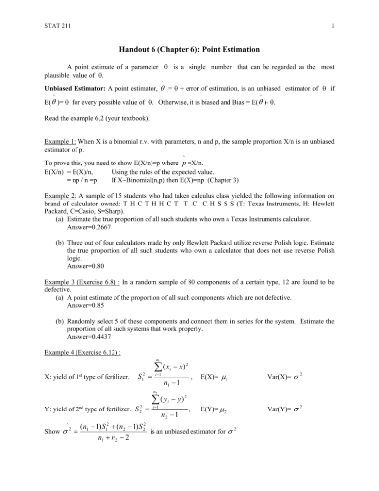
STAT 211
1
Handout 6 (Chapter 6): Point Estimation
A point estimate of a parameter  is a single number that can be regarded as the most
plausible value of .
^
Unbiased Estimator: A point estimator,  =  + error of estimation, is an unbiased estimator of  if
^
^
E(  )=  for every possible value of . Otherwise, it is biased and Bias = E(  )- .
Read the example 6.2 (your textbook).
Example 1: When X is a binomial r.v. with parameters, n and p, the sample proportion X/n is an unbiased
estimator of p.
^
To prove this, you need to show E(X/n)=p where p =X/n.
E(X/n) = E(X)/n,
Using the rules of the expected value.
= np / n =p
If X~Binomial(n,p) then E(X)=np (Chapter 3)
Example 2: A sample of 15 students who had taken calculus class yielded the following information on
brand of calculator owned: T H C T H H C T T C C H S S S (T: Texas Instruments, H: Hewlett
Packard, C=Casio, S=Sharp).
(a) Estimate the true proportion of all such students who own a Texas Instruments calculator.
Answer=0.2667
(b) Three out of four calculators made by only Hewlett Packard utilize reverse Polish logic. Estimate
the true proportion of all such students who own a calculator that does not use reverse Polish
logic.
Answer=0.80
Example 3 (Exercise 6.8) : In a random sample of 80 components of a certain type, 12 are found to be
defective.
(a) A point estimate of the proportion of all such components which are not defective.
Answer=0.85
(b) Randomly select 5 of these components and connect them in series for the system. Estimate the
proportion of all such systems that work properly.
Answer=0.4437
Example 4 (Exercise 6.12) :
n1
X: yield of 1st type of fertilizer.
S12 
 (x
i 1
^
Show  2 
(n1  1) S  (n2  1) S
n1  n2  2
2
1
2
2
 x) 2
,
n1  1
n2
2
Y: yield of 2nd type of fertilizer. S 2 
_
i
(y
i 1
E(X)=  1
Var(X)= 
2
E(Y)=  2
Var(Y)= 
2
_
i
 y) 2
n2  1
,
is an unbiased estimator for 
2
STAT 211
2
 (n1  1) S12  (n2  1) S 22 
   2
n

n

2
1
2


It means that you need to show E 
 (n1  1) S12  (n2  1) S 22 
(n1  1)
(n2  1)
 
E
E S12 
E S 22
n1  n2  2
n1  n2  2

 n1  n2  2
 

 
(n1  1)
(n2  1)
2 
 2  2
n1  n2  2
n1  n2  2
Example 5 (Exercise 6.13) : X1,X2,….,Xn be a random sample from the pdf f(x)=0.5(1+x), -1x1,
^
_
-11. Show that   3 X is an unbiased estimator for  .
^
 
It means that you need show E     .
_
^
E    3 E  X   3 E ( X ) = 
 
  chapter5
where
1
 x2
x3 
1  1   

E ( X )   x  0.5(1  x)dx  0.5
    0.5      ,  1    1
3  1
2 3 2 3 3
 2
1
1
^
The standard error: The standard error of an estimator  is its standard deviation  ^ .

The estimated standard error: The estimated standard error of an estimator is its estimated standard
^
deviation  ^ = s ^ .


The minimum variance unbiased estimator (MVUE): The best point estimate. Among all estimators
^
of  that are unbiased choose the one that has minimum variance. The resulting  is MVUE.
^
^
 
Example 6: If we go back to example 1, the standard error of p is  ^  Var  p  
p
np(1  p ) p(1  p)
Var ( X )
^

Var  p 


2
Chapter3
n
n2
  rulesof var iance n
X ~ Binomial( n , p )
Var ( X )  np (1 p )
^
Example 7: If we go back to example 5, the standard error of  is
 3  2 
Var ( X )
3  2

 
9
 9

n
n
 
 chapter5
 9n 
1  2 3  2

where Var(X)= E ( X 2 )  [ E ( X )] 2  
3 9
9


  Var   9Var X  
^
^
_
1
 x3
x4 
1  1   1
  0.5     

E(X )=  x  0.5(1  x)dx  0.5
4  1
3 4 3 4 3
 3
1
1
2
2
p (1  p )
where
n
STAT 211
3
^
_
Example 8: For normal distribution,   x is the MVUE for . Proof is as follows.
The following graphs are generated by creating 500 samples with size 5 from N(0,1) and calculating the
sample mean and the sample median for each sample.
Example 9 (Exercise 6.3): Given normally distributed data yield the following summary statistics.
Variable
thickness
n
16
Mean
1.3481
Median
1.3950
TrMean
1.3507
Variable
thickness
Minimum
0.8300
Maximum
1.8300
Q1
1.0525
Q3
1.6425
StDev
0.3385
SE Mean
0.0846
(a) A point estimate of the mean value of coating thickness.
(b) A point estimate of the median value of coating thickness.
(c) A point estimate of the value that separates the largest 10% of all values in the coating thickness
distribution from the remaining 90%.
Answer=1.78138
(d) Estimate P(X<1.5) (The proportion of all thickness values less than 1.5)
Answer=0.6736
(e) Estimated standard error of the estimator used in (a).
Answer=0.084625
STAT 211
4
Boxplot of thickness
0.8
1.3
1.8
thickness
Normal Probability Plot for thickness
ML Estimates - 95% CI
99
ML Estimates
95
Mean
1.34812
StDev
0.327781
90
Goodness of Fit
Percent
80
AD*
70
60
50
40
30
1.074
20
10
5
1
0.4
1.4
2.4
Data
METHODS OF OBTAINING POINT ESTIMATORS
1. The Method of Moments (MME)
Let X1,X2,….,Xn be a random sample from a pmf or pdf. For k=1,2,…., the kth population moment
of the distribution is E(Xk). The kth sample moment is
1 n k
 xi .
n i 1
STAT 211
5
Steps to follow : If you have only one unknown parameter
(i)
calculate E(X).
(ii)
1 n 1 _
 xi  x .
n i 1
equate it to
(iii)
Solve for unknown parameter (such as 1).
If you have two unknown parameters, you also need to compute the following to
solve two unknown parameters with two equations.
(iv)
calculate E(X2).
(v)
1 n 2
 xi .
n i 1
equate it to
(vi)
Solve for the second unknown parameter (such as 2).
If you have more than two unknown parameters, repeat the same steps for k=3,….. until you can solve it.
_
Example 10: Show that MME of the parameter  in Poisson distribution is x
There is one unknown parameter.
The 1th population moment of the distribution is E(X)= .
_
The 1th sample moment is
x
_
Then
Example 11:
x
is the MME for 
Find the MME for the parameters  and  in gamma distribution.
There are two unknown parameters.
The 1th population moment of the distribution is E(X)= .
_
The 1th sample moment is
x
_
Then = x but this did not help to solve for any unknown parameter. We need to
continue the steps.
The 2nd population moment of the distribution is E(X2)= 2(1+).
The 2nd sample moment is
Then  2(1+)=
1 n 2
 xi
n i 1
1 n 2
 xi
n i 1
Since we have 2 unknown parameters and two equations, we can solve for the unknown
parameters.
2
_


x

x



i
2
( x)
 , respectively
i 1 
The MME for  and  are
and
2
_
n
_


x
 xi  x 


i 1 
n
_
Example 12:
Find the MME for the parameters  and 2 in normal distribution.
There are two unknown parameters.
The 1th population moment of the distribution is E(X)= .
STAT 211
6
_
The 1th sample moment is x
_
Then = x but we still need to solve for the second unknown parameters. We need to
continue the steps.
The 2nd population moment of the distribution is E(X2)= 2 +2 .
The 2nd sample moment is
1 n 2
 xi
n i 1
1 n 2
Then  + =  xi
n i 1
2
2
Then this can be solved for the second unknown parameter.
2
_


x

x



i
_
 , respectively
i 1 
2
The MME for  and  are x and
n
n
2. The Method of Maximum Likelihood (MLE)
Likelihood function is the joint pmf or pdf of X which is the function of unknown  values when x's
are observed. The maximum likelihood estimates are the  values which maximize the likelihood
function.
Steps to follow:
(i) Determine the likelihood function.
(ii) Take the natural logarithm of the likelihood function.
(iii) Take a first derivative with respect to each unknown  and equate it to zero (if you have m
unknown parameters, you will have m equations as a result of derivatives).
(iv) Solve for unknown 's.
(v)Check if it really maximizes your function by looking at a second derivative.
_
Example 13: Show that MLE of the parameter  in Poisson distribution is x
There is one unknown parameter.
L=Likelihood = p(x1,x2,….,xn) = p(x1)p(x2)….p(xn)
by independence
e    x1 e    x2 e    x3
e    x n e  n   i
=
.
.
……..
= n
x1!
x2 !
x3 !
xn !
 xi !
x
ln(L)=  n 
i 1
 x ln( )   ln( x !)
i
i
d ln( L)
 xi  0 then   x_
 n 
d

d 2 ln( L)
 xi


d2
2
^
_
 0 then the MLE of  is   x

^
^
^
The Invariance Principle: Let  1 .,  2 ,...,  m be the MLE's of the parameters  1 ,  2 ,...,  m . Then the
^
^
^
MLE of any function h(  1 ,  2 ,...,  m ) of these parameters is the function h(  1 .,  2 ,...,  m ) of the MLE's
STAT 211
7
Example 14:
(1) Let X1,…,Xn be a random sample of normally distributed random variables with the mean  and the
standard deviation .
n
_
The method of moment estimates of  and 2 are x and
_
 ( xi  x ) 2
i 1
n
n
_
The maximum likelihood estimates of  and 2 are x and

(n  1) s 2
, respectively
n
_
 ( xi  x ) 2
i 1
n

(n  1) s 2
, respectively
n
(2) Let X1,…,Xn be a random sample of exponentially distributed random variables with parameter .
_
The method of moment estimate and the maximum likelihood estimate of  are 1 / x .
(3) Let X1,…,Xn be a random sample of binomial distributed random variables with parameter p.
The method of moment estimate and the maximum likelihood estimate of p are X/n.
(4) Let X1,…,Xn be a random sample of Poisson distributed random variables with parameter .
_
The method of moment estimate and the maximum likelihood estimate of  are x .
All the estimates above are unbiased? Some Yes but others No. (will be discussed in class)
Example 15 (Exercise 6.20): random sample of n bike helmets are selected.
X: number among the n that are flawed =0,1,2,…..,n
p=P(flawed)
(a) Maximum likelihood estimate (MLE) of p if n=20 and x=3?
(b) Is the estimator in (a) unbiased?
(c) Maximum likelihood of (1-p)5 (none of the next five helmets examined is flawed)?
(d) Instead of selecting 20 helmets to examine, examine the helmets in succession until 3 flawed ones
are found. What would be different in X and p?
Example 16 (Exercise 6.22):
X: the proportion of allotted time that a randomly selected student spends working on a certain aptitude
The pdf of x is f(x;)= (  1) x , 0x1, >-1.
A random sample of 10 students yield the data: 0.92, 0.79, 0.90, 0.65, 0.86, 0.47, 0.73, 0.97, 0.94, 0.77.
(a) Obtain the MME of  and compute the estimate using the data.
1
 x  2 
 1
 
E ( X )   x  (  1) x dx  (  1)
   2 0   2
0
1

_
Set E(X)= x and then solve for .
_
_
~
The given data yield x = 0.80 then the method of moment estimator for  is  
2 x 1
_
1 x

2(0.8)  1
=3
1  0.8
STAT 211
8
(b) Obtain the MLE of  and compute the estimate using the data.
n
L=Likelihood=

i 1
n
n
i 1
i 1
f ( xi )  (  1) xi  (  1) n  xi
ln(L)= n ln(   1)  
n
 ln( x )
i
i 1
n
d ln( L)
n

  ln( xi ) =0 then solve for .
d
  1 i 1
n
The given data yield
 ln( x )  -2.4295
i 1
i
then the maximum likelihood estimator for  is
n
^

n   ln( xi )
i 1
n
  ln( xi )

(10  2.4295)
=3.1161
((2.4295))
i 1
Proposition: Under very general conditions on the joint distribution of the sample when the sample size
is large, the MLE of any parameter  is approximately unbiased and has a variance that is nearly as small
as can be achieved by an estimator.