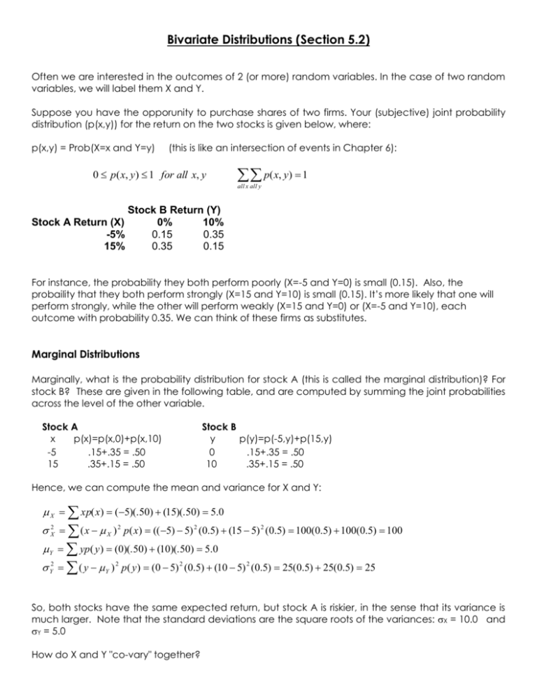
Bivariate Distributions (Section 5.2)
Often we are interested in the outcomes of 2 (or more) random variables. In the case of two random
variables, we will label them X and Y.
Suppose you have the opporunity to purchase shares of two firms. Your (subjective) joint probability
distribution (p(x,y)) for the return on the two stocks is given below, where:
p(x,y) = Prob(X=x and Y=y)
(this is like an intersection of events in Chapter 6):
0  p( x, y)  1 for all x, y
 p( x, y)  1
all x all y
Stock B Return (Y)
Stock A Return (X)
0%
10%
-5%
0.15
0.35
15%
0.35
0.15
For instance, the probability they both perform poorly (X=-5 and Y=0) is small (0.15). Also, the
probaility that they both perform strongly (X=15 and Y=10) is small (0.15). It’s more likely that one will
perform strongly, while the other will perform weakly (X=15 and Y=0) or (X=-5 and Y=10), each
outcome with probability 0.35. We can think of these firms as substitutes.
Marginal Distributions
Marginally, what is the probability distribution for stock A (this is called the marginal distribution)? For
stock B? These are given in the following table, and are computed by summing the joint probabilities
across the level of the other variable.
Stock A
x
p(x)=p(x,0)+p(x,10)
-5
.15+.35 = .50
15
.35+.15 = .50
Stock B
y
p(y)=p(-5,y)+p(15,y)
0
.15+.35 = .50
10
.35+.15 = .50
Hence, we can compute the mean and variance for X and Y:
 X   xp( x)  (5)(. 50)  (15)(. 50)  5.0
 X2   ( x   X ) 2 p( x)  (( 5)  5) 2 (0.5)  (15  5) 2 (0.5)  100(0.5)  100(0.5)  100
 Y   yp( y )  (0)(. 50)  (10)(. 50)  5.0
 Y2   ( y   Y ) 2 p( y )  (0  5) 2 (0.5)  (10  5) 2 (0.5)  25(0.5)  25(0.5)  25
So, both stocks have the same expected return, but stock A is riskier, in the sense that its variance is
much larger. Note that the standard deviations are the square roots of the variances: X = 10.0 and
Y = 5.0
How do X and Y "co-vary" together?
Covariance
COV ( X , Y )  E[( X   X )(Y  Y )]   ( x   X )( y  Y ) p( x, y)   xyp( x, y)   X Y
all x all y
all x all y
For these two firms, we find that the covariance is negative, since high values of X tend to be seen
with low values of Y and vice versa. We compute the Covariance of their returns in the following
table. (X = Y = 5)
x
y
-5
0
-5
10
15
0
15 10
Sum
p(x,y)
.15
.35
.35
.15
xy
0
-50
0
150
x-X
-10
-10
10
10
y-Y
-5
5
-5
5
xyp(x,y)
(x-X)( y-Y)p(x,y)
0(.15)=0
(-10)(-5)(.15)=7.5
-50(.35)=-17.5 (-10)(5)(.35)=-17.5
0(.35)=0
(10)(-5)(.35)=-17.5
150(.15)=22.5
(10)(5)(.15)=7.5
5.0
-20.0
COV(X,Y) = -20.0 = 5.0-(5.0)(5.0)
The negative comes from the fact that when X tends to be large, Y tends to be small and vice versa,
based on the joint probability distribution.
Coefficient of Correlation

COV ( X , Y )
 XY
For the stock data:
COV(X,Y) = -20.0,
X = 10.0,
Y = 5.0,
 = -20/(10*5)=-20/50 = -0.40
Functions of Random Variables
Probability Distribution of the Sum of Two Variables
Suppose you purchase 1 unit of each stock. What is your expected return (in percent). You want the
probability distribuion for the random variable X+Y. Consider the joint probability distribution of X and
Y, and compute X+Y for each outcome.
x
-5
-5
15
15
Sum
y
0
10
0
10
p(x,y)
.15
.35
.35
.15
1.00
x+y
-5+0=-5
-5+10=5
15+0=15
15+10=25
---
(x+y)p(x,y)
(-5)(.15)=-0.75
(5)(.35)=1.75
(15)(.35)=5.25
(25)(.15)=3.75
10.00
(x+y)2p(x,y)
(25)(.15)=3.75
(25)(.35)=8.75
(225)(.35)=78.75
(625)(.15)=93.75
185.00
 X2 Y

 ( x  y)
2
p( x, y)   X2 Y
 185.00  (10.00) 2
 85.00
Thus, the mean, variance, and standard deviation of X+Y (the sum of the returns) are: 10.00, 85.00,
and 9.22, respectively.
Rules for the Mean and Variance of X+Y
E ( X  Y )   X Y   X   Y  E ( X )  E (Y )
V ( X  Y )   X2 Y  V ( X )  V (Y )  2COV ( X , Y )
For the stock return example, we have:
E(X) = 5
E(Y) = 5
V(X) = 100
V(Y) = 25
COV(X,Y) = -20
which gives us:
E(X+Y) = 5+5 = 10
V(X+Y) = 100+25+2(-20)=85
which is in agreement with what we computed by generating the probability distribution for X+Y by
“brute force” above.
Probability Distribution of a Linear Function of Two Variables
Consider a portfolio of two stocks, with Returns (R1,R2), and fixed weights (w1,w2)
Return of portfolio: Rp = w1R1 + w2R2
where w1+w2 = 1, w10, w20
Expected Return on portfolio: E(Rp) = w1E(R1) + w2E(R2)
Variance of Return on Portfolio: V(Rp) = (w1)2V(R1) + (w2)2V(R2) + 2w1w2COV(R1,R2)
Note that the rules for expected value and variance of linear functions does not depend on the
weights summing to 1.
For stock portfolio from two stocks given above, set R1 = X and R2 = Y:
Rp = w1R1 + w2R2 = w1R1 + (1-w1)R2
Expected Return: E(Rp) = w1(5) + (1-w1)(5) = 5
Variance of Return:
V(Rp) = (w1)2(100) + (1-w1)2(25) + 2w1(1-w1)(-20)
Compute the variance if:
i) w1=0.25 and w2=0.75
ii) w1=0.00 and w2=1.00
iii) w1=1.00 and w2=0.00
To minimize the variance of returns, we expand the equation above in terms of w1, take its
derivative with respect to w1, set it equal to 0, and solve for w1:
i)
V(Rp) = 165(w1)2 – 90w1 + 25
ii)
dV(Rp)/dw1 = 2(165)w1 – 90 = 0
iii)
330w1 = 90 ==> w1* = 90/330 = 0.2727
No matter what portfolio we choose, expected returns are 5.0, however we can minimize the
variance of the return (risk) by buying 0.27 parts of Stock A and (1-0.27)=0.73 parts of stock B.
A classic paper on this topic (more mathematically rigorous than this example, where each stock has
only two possible outcomes) is given in: Harry M. Markowitz, ``Portfolio Selection,'' Journal of Finance,
7 (March 1952), pp 77-91.