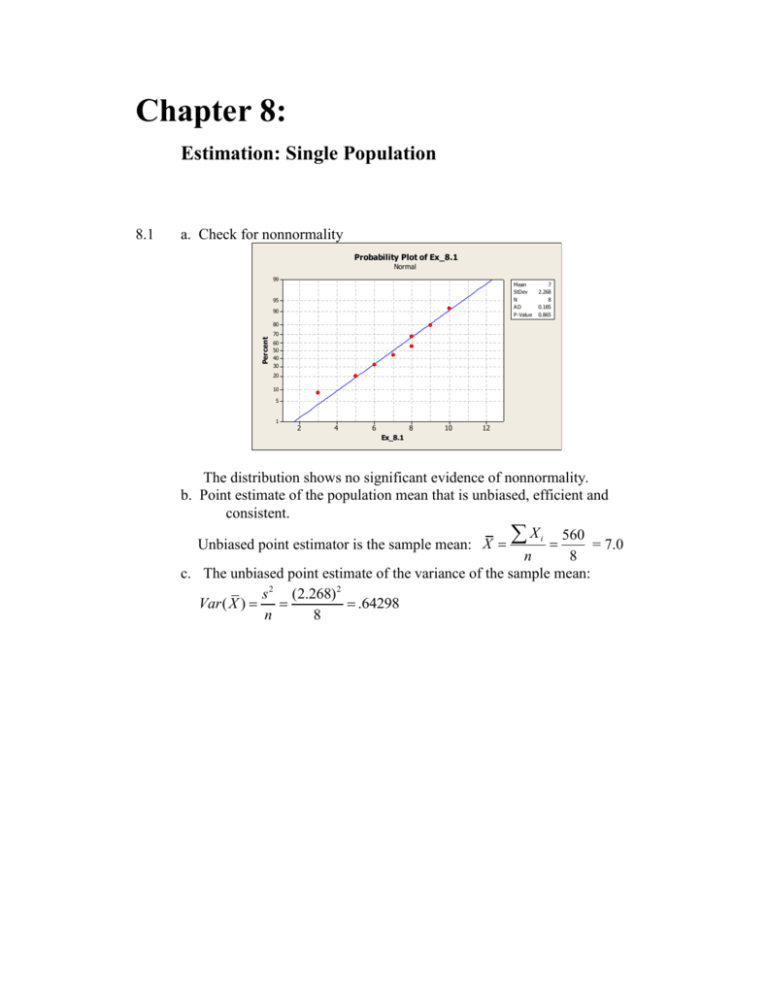
Chapter 8:
Estimation: Single Population
a. Check for nonnormality
Probability Plot of Ex_8.1
Normal
99
Mean
StDev
N
AD
P-Value
95
90
7
2.268
8
0.185
0.865
80
Percent
8.1
70
60
50
40
30
20
10
5
1
2
4
6
8
10
12
Ex_8.1
The distribution shows no significant evidence of nonnormality.
b. Point estimate of the population mean that is unbiased, efficient and
consistent.
 X i  560 = 7.0
Unbiased point estimator is the sample mean: X 
n
8
c. The unbiased point estimate of the variance of the sample mean:
s 2 (2.268) 2
Var ( X )  
 .64298
n
8
164
Statistics for Business & Economics, 6th edition
8.2 a. Evidence of non-normality?
Probability Plot of Homes_Ex8.2
Normal
99
Mean
StDev
N
AD
P-Value
95
90
101.4
14.20
8
0.194
0.837
Percent
80
70
60
50
40
30
20
10
5
1
60
70
80
90
100
110
Homes_Ex8.2
120
130
140
No evidence of non-normality.
b. The minimum variance unbiased point estimator of the population
 X i  560 = 101.375
mean is the sample mean: X 
n
8
c. The unbiased point estimate of the variance of the sample mean:
s 2  201.6964
2
s 2 201.6964
ˆ (X )  
Var ( X ) 
; Var
 25.2121
n
n
8
x 3
d. pˆ    .375
n 8
8.3
n = 10 economists forecast for percentage growth in real GDP in the next
year
Descriptive Statistics: RGDP_Ex8.3
Variable
RGDP_Ex8.3
N
10
N*
0
Variable
RGDP_Ex8.3
Minimum
2.2000
Mean
2.5700
Q1
2.4000
SE Mean
0.0716
TrMean
2.5625
StDev
0.2263
Variance
0.0512
Median
2.5500
Q3
2.7250
Maximum
3.0000
Range
0.8000
CoefVar
8.81
IQR
0.3250
a. Unbiased point estimator of the population mean is the sample mean:
 X i  2.57
X
n
b. The unbiased point estimate of the population variance: s 2  .0512
c. Unbiased point estimate of the variance of the sample mean
s 2 .0512
Var ( X )  
 .00512
n
10
Sum
25.7000
Chapter 8: Estimation: Single Population
x 7

 .70
n 10
e. Unbiased estimate of the variance of the sample proportion:
pˆ (1  pˆ ) .7(1  .7)
Var ( pˆ ) 

 .021
n
10
d. Unbiased estimate of the population proportion: pˆ 
8.4 n = 12 employees. Number of hours of overtime worked in the last month:
a. Unbiased point estimator of the population mean is the sample mean:
 X i  24.42
X
n
b. The unbiased point estimate of the population variance: s 2  85.72
c. Unbiased point estimate of the variance of the sample mean
s 2 85.72
Var ( X )  
 7.1433
n
12
x 3
d. Unbiased estimate of the population proportion: pˆ    .25
n 12
e. Unbiased estimate of the variance of the sample proportion:
pˆ (1  pˆ ) .25(1  .25)
Var ( pˆ ) 

 .015625
n
12
a. Check each variable for normal distribution:
Normal Probability Plot
.999
.99
.95
Probability
8.5
.80
.50
.20
.05
.01
.001
45
50
55
Meals
Average: 50.1
StDev: 2.46842
N: 30
Anderson-Darling Normality Test
A-Squared: 0.413
P-Value: 0.318
165
Statistics for Business & Economics, 6th edition
Normal Probability Plot
.999
.99
Probability
.95
.80
.50
.20
.05
.01
.001
15
20
25
Attendance
Average: 21.24
StDev: 2.50466
N: 25
Anderson-Darling Normality Test
A-Squared: 0.377
P-Value: 0.383
Normal Probability Plot
.999
.99
.95
Probability
166
.80
.50
.20
.05
.01
.001
9
10
11
12
13
14
15
16
Ages
Average: 12.24
StDev: 1.96384
N: 25
Anderson-Darling Normality Test
A-Squared: 0.569
P-Value: 0.126
No evidence of non-normality in Meals, Attendance or Ages
Chapter 8: Estimation: Single Population
167
b. Unbiased estimates of population mean and variance:
Descriptive Statistics: Meals, Attendance, Ages
Variable
Mean
Meals
0.451
Attendan
0.501
Ages
0.393
Variable
Meals
Attendan
Ages
N
Mean
Median
TrMean
StDev
30
50.100
50.000
50.192
2.468
25
21.240
21.000
21.348
2.505
25
12.240
12.000
12.217
1.964
Minimum
45.000
15.000
9.000
Maximum
55.000
25.000
16.000
Q1
48.000
19.500
10.000
Q3
52.000
23.500
14.000
Variable
Unbiased estimate of mean Unbiased estimate of variance (s2)
Meals
50.100
(2.468)2 = 6.0910
Attendance
21.240
(2.505)2 = 6.2750
Ages
12.240
(1.964)2 = 3.8573
8.6
1
1
 
E ( X1 )  E( X 2 )    
2
2
2 2
1
3
 3
E (Y )  E ( X 1 )  E ( X 2 )  

4
4
4 4
1
2
 2
E (Z )  E ( X1 )  E ( X 2 )  

3
3
3 3
2 1
1
12 2
 Var ( X 1 )  Var ( X 2 ) 

b. Var ( X ) 
n 4
4
2 8
4
2
1
9
5
Var (Y )  Var ( X 1 )  Var ( X 2 ) 
16
16
8
2
1
4
5
Var ( Z )  Var ( X 1 )  Var ( X 2 ) 
9
9
9
X is most efficient since Var ( X )  Var (Y )  Var ( Z )
Var (Y ) 5
c. Relative efficiency between Y and X :
  2.5
Var ( X ) 2
Var ( Z ) 20
Relative efficiency between Z and X :

 2.222
Var ( X ) 9
a. E ( X ) 
SE
168
Statistics for Business & Economics, 6th edition
8.7 a. Evidence of non-normality?
Normal Probability Plot for Leak Rates (
ML Estimates
99
ML Estimates
95
Mean
0.0515
StDev
0.0216428
90
Goodness of Fit
Percent
80
AD*
70
60
50
40
30
0.596
20
10
5
1
0.00
0.05
0.10
Data
No evidence of nonnormality exists.
b. The minimum variance unbiased point estimator of the population
 X i  .0515
mean is the sample mean: X 
n
c. The unbiased point estimate of the variance of the sample mean:
s 2 x  (.0216428)2  .0004684
Var ( X ) 
8.8
2
n
ˆ (X ) 
; Var
s 2 .0004684

 .00000937
n
50
a. Evidence of non-normality?
No evidence of the data distribution coming from a non-normal
population
b. The minimum variance unbiased point estimator of the population
 X i  3.8079
mean is the sample mean: X 
n
Descriptive Statistics: Volumes
Variable
Mean
Volumes
0.0118
Variable
Volumes
N
Mean
Median
TrMean
StDev
75
3.8079
3.7900
3.8054
0.1024
Minimum
3.5700
Maximum
4.1100
Q1
3.7400
Q3
3.8700
SE
Chapter 8: Estimation: Single Population
c. Minimum variance unbiased point estimate of the population variance
is the sample variance s2 = .0105
8.9
Reliability factor for each of the following:
a. 96% confidence level: z 2 = +/- 2.05
b. 88% confidence level: z 2 = +/- 1.56
c. 85% confidence level: z 2 = +/- 1.44
d.   .07 z 2 = +/- 1.81
e.  2 = .07 z 2 = +/- 1.48
8.10 Calculate the margin of error to estimate the population mean
a. 98% confidence level; n = 64, variance = 144
 = 3.495
= 2.33 12
ME  z 2 

n
64 

b. 99% confidence interval, n=120; standard deviation = 100
 = 23.552
ME  z 2 
= 2.58 100

n
120 

8.11 Calculate the width to estimate the population mean, for
a. 90% confidence level, n = 100, variance = 169
  = 4.277
 = 2 1.645 13
width = 2ME = 2  z 2 



100  
n 



b. 95% confidence interval, n = 120, standard deviation = 25
  = 8.9461
 = 2 1.96  25
width = 2ME = 2  z 2 



120  
n 



8.12
Calculate the LCL and UCL
 = 40.2 to 59.8
a. x  z 2 
= 50  1.96  40

n
64 

 = 81.56 to 88.44
b. x  z 2 
= 85  2.58  20

n
225 

 = 506.2652 to 513.73478
c. x  z 2 
= 510  1.645  50

n
485 

8.13 a. n  9, x  187.9,   32.4, z.10  1.28
187.9  1.28(32.4/3) = 174.076 up to 201.724
b. 210.0 – 187.9 = 22.1 = z / 2 (32.4 / 3), z / 2  2.05
  2[1  Fz (2.05)]  .0404
100(1-.0404)% = 95.96%
169
170
Statistics for Business & Economics, 6th edition
8.14 a. Find the reliability factor for 92% confidence level: z 2 = +/- 1.75
b. Calculate the standard error of the mean

= .63246
 6
n
90
c. Calculate the width of the 92% confidence interval for the population
mean
  = 2.2136
 = 2 1.75  6
width = 2ME = 2  z 2 




90
n





8.15 a. n  25, x  2.90,   .45, z.025  1.96
 = 2.90  1.96(.45/5) = 2.7236 up to 3.0764
x  z  

n

b. 2.99 – 2.90 = .09 = z / 2 (.45 / 5), z / 2  1
  2[1  Fz (1)]  .3174
100(1-.3174)% = 68.26%
8.16 a. n  16, x  4.07,   .12, z.005  2.58
4.07  2.58(.12/4) = 3.9926 up to 4.1474
b. narrower since the z score for a 95% confidence interval is smaller
than the z score for the 99% confidence interval
c. narrower due to the smaller standard error
d. wider due to the larger standard error
8.17 Find the reliability factor tv ,
a.
b.
c.
d.
2
n = 20, 90% confidence level; t = 1.729
n = 7, 98% confidence level; t = 3.143
n = 16, 95% confidence level; t = 2.131
n = 23, 99% confidence level; t = 2.819
8.18 Find the ME
a. n = 20, 90% confidence level, s = 36
 = 13.9182
ME  t 2 s
= ME  1.729  36

n
120 

b. n = 7, 98% confidence level, s = 16
ME  t 2 s
= ME  3.143 16  = 19.007
n
7

c. n = 16, 99% confidence level, x1 = 15, x2 = 17, x3 = 13, x4 = 11, x5 = 14
 = 7.5407
x  14, s  2.58199 ME  5.841 2.58199

4

Chapter 8: Estimation: Single Population
8.19 Time spent driving to work for n = 5 people
Descriptive Statistics: Driving_Ex8.19
Variable
Sum
Driving_Ex8.19
192.00
N
N*
Mean
SE Mean
TrMean
StDev
Variance
CoefVar
5
0
38.40
2.66
*
5.94
35.30
15.47
Variable
Driving_Ex8.19
Minimum
30.00
Q1
32.50
Median
40.00
Q3
43.50
Maximum
45.00
Range
15.00
IQR
11.00
a. Calculate the standard error
s
2.6571
 5.94138
n
5
b. Find the value of t for the 95% confidence interval
tv , 2 = 2.776
c. Calculate the width for a 95% confidence interval for the population mean
ME  t 2 s
= ME  2.776  5.94138  = 14.752
n
5

8.20 Find the LCL and UCL for each of the following:
a. alpha = .05, n = 25, sample mean = 560, s = 45
 = 560  2.064  45
 = 541.424 to 578.576
x  t 2  s



n
25




b. alpha/2 = .05, n = 9, sample mean = 160, sample variance = 36
 = 160  1.860  6  = 156.28 to 163.72
x  t 2  s



n
9


c. 1   = .98, n = 22, sample mean = 58, s = 15
 = 58  2.518 15
 = 49.9474 to 66.0526
x  t 2  s



n
22




8.21 Calculate the margin of error to estimate the population mean for:
a. 98% confidence level; n = 64, sample variance = 144
 = 3.585
ME  t 2 s
= ME  2.390 12

n
64 

b. 99% confidence level; n = 120, sample standard deviation = 100
 = 24.2824
ME  t 2 s
= ME  2.660 100

n
120 

c. 95% confidence level; n = 200, sample standard deviation = 40
 = 5.65685
ME  t 2 s
= ME  2.000  40

n
200 

171
172
Statistics for Business & Economics, 6th edition
8.22 Calculate the width for each of the following:
a. alpha = 0.05, n = 6, s = 40
w  2ME  2t  2 s
 2  2.571 40   2(41.98425)  83.9685
n
6

b. alpha = 0.01, n = 22, sample variance = 400
  2(12.07142)  24.1428
w  2ME  2t  2 s
 2  2.831 20

n
22 

c. alpha = 0.10, n = 25, s = 50
  2(17.11)  34.22
w  2ME  2t  2 s
 2  1.711 50

n
25


8.23 a. 95% confidence interval:
Results for: TOC.xls
One-Sample T: Leak Rates (cc/sec.)
Variable
Leak Rates (
N
50
Mean
0.05150
StDev
0.02186
SE Mean
0.00309
95.0% CI
( 0.04529, 0.05771)
b. 98% confidence interval:
One-Sample T: Leak Rates (cc/sec.)
Variable
Leak Rates (
N
50
Mean
0.05150
StDev
0.02186
SE Mean
0.00309
98.0% CI
( 0.04406, 0.05894)
8.24 a.
Results for: Sugar.xls
Descriptive Statistics: Weights
Variable
Mean
Weights
0.95
Variable
Weights
N
Mean
Median
TrMean
StDev
100
520.95
518.75
520.52
9.45
Minimum
504.70
Maximum
544.80
Q1
513.80
Q3
527.28
SE
90% confidence interval:
Results for: Sugar.xls
One-Sample T: Weights
Variable
Weights
N
100
Mean
520.948
StDev
9.451
SE Mean
0.945
90.0% CI
( 519.379, 522.517)
b. narrower since a smaller value of z will be used in generating the 80%
confidence interval.
8.25
n  9, x  157.82, s  38.89, t8,.025  2.306
margin of error:  2.306(38.89/3) =  29.8934
8.26
n  7, x  74.7143, s  6.3957, t6,.025  2.447
margin of error:  2.447(6.3957/ 7 ) =  5.9152
Chapter 8: Estimation: Single Population
8.27
a. n  10, x  15.90, s  5.30, t9,.005  3.25
15.90  3.25(5.30/ 10 ) = 10.453 up to 21.347
b. narrower since the t-score will be smaller for a 90% confidence
interval than for a 99% confidence interval
8.28
n  25, x  42, 740, s  4, 780, t24,.05  1.711
42,740  1.711(4780/5) = $41,104.28 up to $44,375.72
8.29
n  9, x  16.222, s  4.790, t8,.10  1.86
We must assume a normally distributed population
16.222  1.86(4.790/3) = 13.252 up to 19.192
8.30 Find the standard error of the proportion for
pˆ (1  pˆ )
.3(.7)
a. n = 250, p̂ = 0.3
= .02898

n
250
pˆ (1  pˆ )
.45(.55)
b. n = 175, p̂ = 0.45
= .03761

n
175
pˆ (1  pˆ )
.05(.95)
c. n = 400, p̂ = 0.05
= .010897

n
400
8.31 Find the margin of error for
a. n = 250, p̂ = 0.3, α = .05 z 2
b. n = 175, p̂ = 0.45, α = .08 z 2
c. n = 400, p̂ = 0.05, α = .04 z 2
pˆ (1  pˆ )
.3(.7)
= .056806
 1.96
n
250
pˆ (1  pˆ )
.45(.55)
= .05810
 1.75
n
175
pˆ (1  pˆ )
.05(.95)
= .02234
 2.05
n
400
8.32 Find the confidence level for estimating the population proportion for
a. 92.5% confidence level; n = 650, p̂ = .10
pˆ (1  pˆ )
.10(1  .10)
= .10  1.78
= .079055 to .120945
n
650
b. 99% confidence level; n = 140, p̂ = .01
pˆ  z 2
pˆ (1  pˆ )
.01(1  .01)
= .01  2.58
= 0.0 to .031696
n
140
c. alpha = .09; n = 365, p̂ = .50
pˆ  z 2
pˆ  z 2
pˆ (1  pˆ )
.5(.5)
= .50  1.70
= .4555 to .5445
n
650
173
174
8.33
8.34
Statistics for Business & Economics, 6th edition
n = 142, 87 answered GMAT or GRE is ‘very important’. 95% confidence
interval for the population proportion:
.61268(1  .61268)
pˆ (1  pˆ )
= .61268  1.96
= .53255 to .6928
pˆ  z 2
142
n
n  95,
pˆ  67 / 95  .7053, z.005  2.58
pˆ (1  pˆ )
.7053(.2947)
= .7053  (2.58)
=
n
95
99% confidence interval: .5846 up to .8260
pˆ  z / 2
8.35 a. unbiased point estimate of proportion:
Tally for Discrete Variables: Adequate Variety
Adequate Variety
1
2
N=
Count CumCnt
135
135
221
356
356
Percent CumPct
37.92 37.92
62.08 100.00
x 135

 .3792
n 356
b. 90% confidence interval:
n  356, pˆ  135 / 356  .3792, z.05  1.645
pˆ 
pˆ (1  pˆ )
= .3792  (1.645) .3792(.6208) / 356 =
n
.3369 up to .4215
pˆ  z / 2
8.36
n  320,
pˆ  80 / 320  .25, z.025  1.96
pˆ (1  pˆ )
= .25  (1.96) .25(.75) / 320 =
n
95% confidence interval: .2026 up to .2974
pˆ  z / 2
8.37
n  400,
pˆ  320 / 400  .80, z.01  2.326
pˆ (1  pˆ )
.80(1  .80)
= .80  2.326
= .75348
n
400
b. width of a 90% confidence interval
pˆ (1  pˆ )
.8(1  .8)
w  2ME  2 z 2
 2  1.645
 2(.0329)  .0658
n
400
a. LCL = pˆ  z / 2
Chapter 8: Estimation: Single Population
8.38
width = .545-.445 = .100; ME = 0.05 pˆ  0.495
pˆ (1  pˆ )
.495(.505)

 .0355
n
198
.05 = z / 2 (.0355), z / 2  1.41
  2[1  Fz (1.41)]  .0793
100(1-.1586)% = 84.14%
8.39
n  420,
pˆ  223/ 420  .5310, z.025  1.96
pˆ (1  pˆ )
= .5310  (1.96) .5310(.4690) / 420 =
n
95% confidence interval: .4833 up to .5787
The margin of error is .0477
pˆ  z / 2
8.40
n  246,
pˆ  40 / 246  .1626, z.01  2.326
pˆ (1  pˆ )
= .1626  (2.326) .1626(.8374) / 246 =
n
98% confidence interval: .1079 up to .2173
pˆ  z / 2
8.41
a. n  246,
pˆ  232 / 246  .9431, z.01  2.326
pˆ (1  pˆ )
= .9431  (2.326) .9431(.0569) / 246 =
n
98% confidence interval: .9087 up to .9775
b. n  246, pˆ  10 / 246  .0407, z.01  2.326
pˆ  z / 2
pˆ (1  pˆ )
= .0407  (2.326) .0407(.9593) / 246 =
n
98% confidence interval: .0114 up to .0699
pˆ  z / 2
8.42
a. n  10, x  257, s  37.2, t9,.05  1.833
 = 257  1.833(37.2/ 10 ) = 235.4318 up to 278.5628
x  t 2  s

n


assume that the population is normally distributed
b. 95% and 98% confidence intervals:
 = 257  2.262(37.2/ 10 ) = 230.39 up to 283.61
[95%]: x  t 2  s

n


 = 257  2.821(37.2/ 10 ) = 223.815 up to
[98%]: x  t 2  s

n


290.185
175
176
Statistics for Business & Economics, 6th edition
n  16, x  150, s  12, t15,.025  2.131
8.43
 = 150  2.131(12/4) = 143.607 up to 156.393
x  t 2  s

n

It is recommended that he stock 157 gallons.
n  50, x  30, s  4.2, z.05  1.645
8.44
= 30  1.645(4.2/ 50 ) = 29.0229 up to 30.9771
8.45
Results from Minitab:
Descriptive Statistics: Passengers8_45
Variable
Mean
Passenge
3.46
Variable
Passenge
N
Mean
Median
TrMean
StDev
50
136.22
141.00
136.75
24.44
Minimum
86.00
Maximum
180.00
Q1
118.50
Q3
152.00
One-Sample T: Passengers8_45
Variable
Passengers8_
N
50
Mean
136.22
StDev
24.44
SE Mean
3.46
(
95.0% CI
129.27, 143.17)
95% confidence interval: 129.27 up to 143.17
8.46
a. Use a 5% risk. Incorrect labels = 8/48 = 0.1667
0.1667(0.8333)
0.1667  1.96
 0.1667  0.1054 = 0.0613 up to 0.2721
48
b. For a 90% confidence interval,
0.1667(0.8333)
0.1667  1.645
 0.1667  0.0885 = 0.0782 up to
48
0.2552
8.47
a. The minimum variance unbiased point estimator of the population
 X i  27  3.375. The unbiased point
mean is the sample mean: X 
n
8
2
 xi  nx 2  94.62  8(3.375)2  .4993
estimate of the variance: s 2 
n 1
7
x 3
b. pˆ    .375
n 8
8.48
3.69 – 3.59 = 0.10 = z / 2 (1.045/ 457), z / 2  2.05
  2[1  Fz (2.05)]  .0404
100(1-.0404)% = 95.96%
SE
Chapter 8: Estimation: Single Population
8.49
n  174,
x  6.06, s  1.43
6.16 – 6.06 = .1 = z / 2 (1.43/ 174), z / 2  .922
  2[1  Fz (.92)]  .3576
100(1-.3576)% = 64.24%
8.50 n = 33 accounting students who recorded study time
a. An unbiased, consistent, and efficient estimator of the population mean
is the sample mean x = 8.545
b. Find the sampling error for a 95% confidence interval; Using degrees of
freedom = 30,
 = 1.3568
ME  2.042  3.817

33 

8.51 n = 25 patient records – the average length of stay is 6 days with a standard
deviation of 1.8 days
a. find the reliability factor for a 95% interval estimate t / 2  2.064
b. Find the LCL for a 99% confidence interval estimate of the population
mean
 . The LCL = 5.257
ME  t 2 s
= 6  2.064 1.8

n
25 

8.52 n = 250, x = 100
a. Find the standard error to estimate population proportion of first timers
pˆ (1  pˆ )
.4(1  .4)
= .03098

n
250
b. Find the sampling error. Since no confidence level is specified, we find
the sampling error (Margin of Error) for a 95% confidence interval.
ME = 1.96 (0.03098) = 0.0607
c. For a 92% confidence interval,
ME = 1.75 (0.03098) = 0.05422
0.40  .05422 giving 0.3457 up to 0.4542
8.53
8.54
a. 90% confidence interval reliability factor = t / 2  1.729
b. Find the LCL for a 99% confidence interval
LCL = 60.75 – 2.861 21.83159
= 46.78 or approximately 47
20
passengers.
a. Find a 95% confidence interval estimate for the population proportion
of students who would like supplements in their smoothies.
177
178
Statistics for Business & Economics, 6th edition
Tally for Discrete Variables: Supplements, Health Consciousness
Supplements
No
0
Yes
1
N=
n  113,
Count
42
71
113
Percent
37.17
62.83
Health
Consciousness
Very
1
Moderately 2
Slight
3
Not Very
4
N=
Count
29
55
20
9
113
Percent
25.66
48.67
17.70
7.96
pˆ  71/113  .62832, z.05  1.96
pˆ (1  pˆ )
.62832(1  .62832)
= .62832  1.96
n
113
0.0891 = 0.5392 up to 0.71742.
pˆ  z / 2
= 0.62832 ±
b. pˆ  29 / 113  0.2566 For 98% confidence level,
pˆ  2.33
(0.2566)(1  0.2566)
 0.2566  0.09573
113
or 0.1609 up to
0.3523
c. pˆ  77 / 113  0.6814
0.6814  1.645
(0.6814)(1  0.6814)
 0.6814  0.0721 or 0.6093 up to
113
0.7535
8.55
n = 100 students at a small university.
a. Estimate the population grade point average with 95% confidence level
One-Sample T: GPA
Variable
GPA
N
100
Mean
3.12800
StDev
0.36184
SE Mean
0.03618
95% CI
(3.05620, 3.19980)
b. Estimate the population proportion of students who were very dissatisfied
(code 1) or moderately dissatisfied (code 2) with parking. Use a 90%
confidence level.
Tally for Discrete Variables: Parking
Parking
1
2
3
4
5
N=
Count
19
26
18
18
19
100
n  100,
Percent
19.00
26.00
18.00
18.00
19.00
pˆ  45 /100  .45, z.05  1.645 , pˆ  z / 2
.45  1.645
pˆ (1  pˆ )
n
.45(1  .45)
= .45 ± .08184 = .368162 up to .53184
100
c. Estimate the proportion of students who were at least moderately
satisfied
(codes 4 and 5) with on-campus food service
Chapter 8: Estimation: Single Population
179
Tally for Discrete Variables: Dining
Dining
1
2
3
4
5
N=
Count
14
26
21
20
19
100
Percent
14.00
26.00
21.00
20.00
19.00
n  100,
pˆ  39 /100  .39, z.05  1.645
pˆ  z / 2
pˆ (1  pˆ )
.39(1  .39)
= .39  1.645
= .39 ± .08023 = .30977 up
n
100
to .47023.
8.56
a. Estimate the average age of the store’s customers by the sample mean
 xi  6310  50.48
x
n
125
To find a confidence interval estimate we will assume a 95% confidence level:
13.06
50.48  1.96
 50.48  2.29 ; 48.19 up to 52.77 years
125
b. Estimate the population proportion of customers dissatisfied with the delivery
system
Tally for Discrete Variables: Dissatisfied with Delivery
Dissatisfied
with
Delivery
1
2
N=
Count
9
116
125
Percent
7.20
92.80
pˆ  9 /125  .072 ; Assuming a 95% confidence level, we find:
0.072  1.96
(0.072)(1  0.072)
 0.072  0.0453 or 0.0267 up to 0.1173
125
c. Estimate the population mean amount charged to a Visa credit card
Descriptive Statistics: Cost of Flowers
Variable
Cost of Flowers
Method of
Payment
American Express
Cash
Master Card
Other
Visa
Mean
52.99
51.34
54.58
53.42
52.65
SE Mean
2.23
4.05
3.11
2.99
2.04
TrMean
52.83
51.46
54.43
53.72
52.58
StDev
10.68
16.19
15.25
14.33
12.71
The population mean can be estimated by the sample mean amount
charged to a Visa credit card = $52.65.
8.57 n = 500 motor vehicle registrations, 200 were mailed, 160 paid in person,
remainder paid on-line.
a. Estimate the population proportion to pay for vehicle registration
renewals in person, use a 90% confidence level.
Median
50.55
50.55
55.49
54.85
50.65
180
Statistics for Business & Economics, 6th edition
Test and CI for One Proportion
Test of p = 0.5 vs p not = 0.5
Sample
X
N Sample p
90% CI
1
160 500 0.320000 (0.285686, 0.354314)
The 90% confidence interval is from 28.56856% up to 35.4314%
b. Estimate the population proportion of on-line renewals, use 95%
confidence.
Test and CI for One Proportion
Test of p = 0.5 vs p not = 0.5
Sample
X
N Sample p
95% CI
1
140 500 0.280000 (0.240644, 0.319356)
The 95% confidence interval is from 24.0644% up to 31.9356%
8.58
From the data in 8.57, find the confidence level if the interval extends
from 0.34 up to 0.46.
ME = ½ the width of the confidence interval. 0.46 – 0.34 = 0.12 / 2 =
0.06
pˆ (1  pˆ )
or
ME  z  2
n
(0.4)(0.6)
0.06  z  2
500
Solving for z: z  2  2.74
Area from the z-table = .4969 x 2 = .9938. The confidence level is
99.38%
8.59 From the data in 8.57, find the confidence level if the interval extends from
23.7% up to 32.3%. ME = ½ the width of the confidence interval. .323 –
.237 = .086 / 2 = .043 and pˆ  .28
pˆ (1  pˆ )
.28(1  .28)
solving for z: z 2  2.14
.043  z 2
n
500
Area from the z-table = .4838 x 2 = .9676. The confidence level is
96.76%
ME  z 2
8.60
a. What is the margin of error for a 99% confidence interval
pˆ (1  pˆ )
pˆ  x  250
 .7143 ,
ME  z 2
n
350
n
.7143(1  .7143)
ME  2.58
350
ME = .0623
=
Chapter 8: Estimation: Single Population
b. Is the margin of error for a 95% confidence larger, smaller or the same as the
99% confidence level? The margin of error will be smaller (more
precise)
for a lower confidence level. The difference in the equation is the
value for z
which would drop from 2.58 down to 1.96.
8.61 Compute the 98% confidence interval of the mean age of on-line renewal
users. n= 460, sample mean = 42.6, s = 5.4.
 = 42.6 ± .58664 = 42.0134 up to
= 42.6  2.33  5.4
x  t 2 s

n
460


43.18664
181