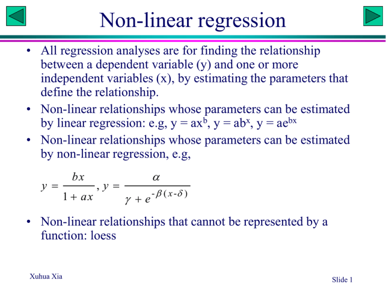
Non-linear regression
• All regression analyses are for finding the relationship
between a dependent variable (y) and one or more
independent variables (x), by estimating the parameters that
define the relationship.
• Non-linear relationships whose parameters can be estimated
by linear regression: e.g, y = axb, y = abx, y = aebx
• Non-linear relationships whose parameters can be estimated
by non-linear regression, e.g,
y 
bx
1  ax
,y 

 e
-  ( x - )
• Non-linear relationships that cannot be represented by a
function: loess
Xuhua Xia
Slide 1
Growth curve of E. coli
• A researcher wishes to estimate the growth curve of
E. coli. He put a very small number of E. coli cells
into a large flask with rich growth medium, and take
samples every half an hour to estimate the density
(n/L).
• 14 data points over 7 hours were obtained.
• What is the instantaneous rate of growth (r). What is
the initial density (N0)?
• As the flask is very large, he assumed that the
growth should be exponential, i.e., y = a·ebx (Which
parameter correspond to r and which to N0?)
• Three approaches
– Log-Transform to linear relationship
– Direct least-square solution (EXCEL solver)
– Direct least-absolute-difference solution (EXCEL solver)
Xuhua Xia
Time
Density
1
20.023
2
39.833
3
80.571
4
161.102
5
317.923
6
635.672
7
1284.54
8
2569.43
9
5082.65
10
10220.8
11
20673.9
12
40591.4
13
81374.6
14
163964
Slide 3
Scatter plot
180000
D  D0e
Density
160000
y = 10.016e0.6928x
R2 = 1
rt
140000
In EXCEL:
120000
Log-transform D
Run linear regression
Obtain D0 and r
100000
80000
60000
40000
20000
0
1
3
5
7
9
11
13
Time
Xuhua Xia
Slide 4
EXCEL solver
Time
Density
Pred
SS
a 9.554915
Pred
SAD
a 9.554956
1
20.023
39.833
80.571
161.102
317.923
635.672
1284.54
2569.43
5082.65
10220.8
20673.9
40591.4
81374.6
163964
19.172
0.724
b 0.696402
19.173
0.850
b 0.696453
38.469
1.860
38.473
1.360
77.189
11.436
77.201
3.370
154.882
38.690
154.914
6.188
310.774
51.115
310.854
7.069
623.573
146.380
623.767
11.905
1251.212
1111.019
1251.666
32.878
2510.582
3463.120
2511.621
57.809
5037.532
2036.008
5039.875
42.779
10107.907
12739.579
10113.126
107.651
20281.716 153787.323
20293.226
380.647
40695.664
10862.758
40720.843
129.404
81656.653
79530.444
81711.360
336.718
163845.689
13967.378
277747.832
163963.851
0.022
1118.648
2
3
4
5
6
7
8
9
10
11
12
13
14
Get initial value for r:
D2
D1

D0e
rt 2
D0e
rt1

D0e
r ( t1  1)
D0e
rt1
rt

D0e 1 e
D0e
rt1
r
e
r
Initial value for D0 is obtained with t = 0
Xuhua Xia
Slide 5
Body weight of wild elephant
• A researcher wishes to estimate the body weight of wild
elephants.
• He measured the body weight of 13 captured elephants of
different sizes as well as a number of predictor variables, such
as leg length, trunk length, etc. Through stepwise regression,
he found that the inter-leg distance (shown in figiure) is the
best predictor of body weight.
• He learned from his former biology professor that the
allometric law governing the body weight (W) and the length
of a body part (L) states that
W = aLb
• Use the three approaches to fit
the equation
Xuhua Xia
Slide 6
Scatter plot
W = aLb
In EXCEL:
50
Log-transform W and L
Run linear regression
Obtain a and b
40
W
y = 20.018x 2.1382
R2 = 0.9955
30
20
10
0
0.2
0.4
0.6
0.8
1
1.2
1.4
L
Xuhua Xia
Slide 7
EXCEL solver
L
0.3
0.4
0.5
0.6
0.7
0.8
0.9
1
1.1
1.2
1.3
1.4
1.5
Xuhua Xia
W
1.657
2.500
4.680
7.075
10.070
11.988
14.836
18.318
23.496
27.897
36.796
44.611
50.183
Pred
1.165
2.285
3.853
5.904
8.471
11.580
15.258
19.527
24.409
29.924
36.093
42.932
50.459
251.859
SS
0.242
0.046
0.684
1.370
2.557
0.166
0.178
1.461
0.833
4.111
0.495
2.820
0.076
15.039
a 19.52661
b 2.341457
W=aLb
Initial values:
W2

W1
L 
 2 
aL
 L1 
b
2
b
1
b
aL
W 
L 
ln  2   b ln  2 
 W1 
 L1 
a 
W
b
L
Slide 8
DNA and protein gel electrophoresis
• How to estimate the molecular
mass of a protein?
– A ladder: proteins with known
molecular mass
– Deriving a calibration curve
relating molecular mass (M) to
migration distance (D): D =
F(M)
– Measure D and obtain M
• The calibration curve is
obtained by fitting a regression
model
Xuhua Xia
Slide 9
Protein molecular mass
• The equation D=aebM appears to describe the
relationship between D and M quite well. This
relationship is better than some published
relationships, e.g.,
D = a – b ln(M)
• The data are my measurement of D and M for a
subset of secreted proteins from the gastric
pathogen Helicobacter pylori (Bumann et al.,
2002).
• Homework: use the data and the three
approaches to estimate parameters a and b (You
don’t need to submit)
Mass
D
5
14.5
10
12.6
20
9.4
30
7.1
40
5.3
50
3.9
60
3.05
70
2.3
80
1.75
Bumann, D., Aksu, S., Wendland, M., Janek, K., Zimny-Arndt, U., Sabarth, N., Meyer, T.F., and
Jungblut, P.R., 2002, Proteome analysis of secreted proteins of the gastric pathogen Helicobacter pylori.
Infect. Immun. 70: 3396-3403.
Xuhua Xia
Slide 10
Area and Radius
What is the functional relationship between the area
and the radius?
Homework (you do not need to submit): Measure the
area A (by counting the squares) and radius r for each
circle and estimate the parameters c and d in the
equation A = crd by using the three approaches.
Xuhua Xia
Toxicity study: pesticide
100
90
Percentage killed
80
70
60
50
40
30
20
10
0
25
30
35
40
45
50
55
60
65
70
Dosage
What transformation to use?
Xuhua Xia
Slide 12
Probit and probit transformation
• Probit has two names/definitions, both
associated with standard normal
distribution:
– the inverse cumulative distribution
function (CDF)
– quantile function
0.9
0.8
0.7
0.6
CDF
• CDF is denoted by (z), which is a
continuous, monotone increasing
sigmoid function in the range of (0,1),
e.g.,
(z) = p
(-1.96) = 0.025 = 1 - (1.96)
• The probit function gives the 'inverse'
computation, formally denoted -1(p),
i.e.,
probit(p) = -1(p)
probit(0.025) = -1.96 = -probit(0.975)
• [probit(p)] = p, and probit[(z)] = z.
1
0.5
0.4
0.3
0.2
0.1
0
-2.5
-1.5
-0.5
0.5
1.5
z
Xuhua Xia
Slide 13
Data
Dosage
Xuhua Xia
27
28
31
31
35
36
37
38
38
40
41
43
44
44
44
45
45
45
46
46
46
47
47
48
49
49
49
49
50
50
51
%Killed
0.9
1.39
2.4
2.49
6.42
7.78
9.16
10.21
11.71
16.24
16.9
22.94
27.35
27.45
28.14
28.97
29.96
30.5
34.3
35.39
35.65
37.55
38.46
40.97
44.37
45.71
46.66
47.38
49.86
52.26
55.12
Probit
Pred
PredOriginalSUMMARY OUTPUT
-2.365618 -2.354331 0.927805
-2.200097 -2.251524 1.217619 Regression Statistics
-1.977368 -1.943104 2.600181 Multiple R 0.999559
-1.961678 -1.943104 2.600181 R Square
0.999118
-1.520442 -1.531877 6.277642 Adjusted R Square
0.999103
-1.420026
-1.42907 7.649205 Standard Error
0.029949
-1.330967 -1.326263 9.237624 Observations
60
-1.269676 -1.223457 11.05786
-1.189609 -1.223457 11.05786 ANOVA
-0.984642 -1.017843 15.43762
df
-0.958124 -0.915036 18.00863 Regression
-0.740824 -0.709423
23.9031 Residual
-0.602262 -0.606616 27.20528 Total
SS
MS
1 58.94878 58.94878
F
65722.54954
Significance F
2.71096E-90
58 0.052022 0.000897
59 59.00081
-0.599259 -0.606616 27.20528
-0.578688 -0.606616 27.20528
Coefficients
Standard Error t Stat
P-value
-0.554261
-0.50381 30.71976 Intercept
-5.130112 0.020381 -251.7115
7.83524E-90
-0.525551
-0.50381 30.71976 Dosage
0.102807 0.000401 256.3641
2.71096E-90
-0.510073
-0.50381 30.71976
-0.404289 -0.401003
34.4209
-0.374812 -0.401003
34.4209
-0.36783 -0.401003
34.4209
-0.317321 -0.298196 38.27768
-0.293421 -0.298196 38.27768
-0.228317 -0.195389 42.25441
-0.141595 -0.092583 46.31176
-0.107742 -0.092583 46.31176
-0.083819 -0.092583 46.31176
-0.065721 -0.092583 46.31176
-0.003509 0.010224 50.40788
0.05668 0.010224 50.40788
0.128694 0.113031 54.49969
Slide 14
Non-linear regression
• In rapidly replicating unicellular eukaryotes such as
the yeast, highly expressed intron-containing genes
requires more efficient splicing sites than lowly
expressed genes.
• Natural selection will operate on the mutations at the
slicing sites to optimize splicing efficiency.
• Designate splicing efficiency as SE and gene
expression as GE.
• Certain biochemical reasoning suggests that SE and
GE will follow the following relationships:
Xuhua Xia
GE
SE
1
0.46
2
0.47
3
0.57
4
0.61
5
0.62
6
0.68
7
0.69
8
0.78
9
0.7
10
0.74
11
0.77
12
0.78
13
0.74
13
0.8
15
0.8
16
0.78
Slide 16
Scatter plot
0.9
0.8
SE
0.7
0.6
SE 
0.5
   GE
1   GE
0.4
0.3
0
2
4
6
8
10
12
14
16
GE
Initial values:
Xuhua Xia
  0.4 (inferred when GE = 0)
/  1 or    (inferred when GE is very large)
When GE = 8, we have (0.4+8 )/(1+8 ) = 0.78
Slide 17
EXCEL: Solver
GE
1
2
3
4
5
6
7
8
9
10
11
12
13
13
15
16
SE
0.46
0.47
0.57
0.61
0.62
0.68
0.69
0.78
0.7
0.74
0.77
0.78
0.74
0.8
0.8
0.78
Pred
0.436655
0.510256
0.565294
0.608005
0.642114
0.669981
0.693177
0.712784
0.729577
0.74412
0.756837
0.768052
0.778016
0.778016
0.794944
0.802195
Xuhua Xia
SS
Alpha 0.333196
0.000544981
Beta 0.192031
0.00162052 Gamma 0.202841
2.21506E-05
3.98053E-06
0.000489015
0.000100378
1.00918E-05
0.004517926
0.000874801
1.69749E-05
0.000173259
0.000142753
0.001445212
0.000483299
2.55629E-05
0.000492612
0.010963515
SE 
   GE
1   GE
Slide 18