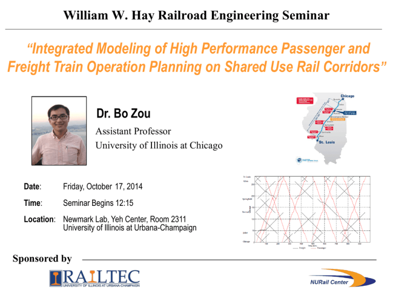
William W. Hay Railroad Engineering Seminar
“Integrated Modeling of High Performance Passenger and
Freight Train Operation Planning on Shared Use Rail Corridors”
Dr. Bo Zou
Assistant Professor
University of Illinois at Chicago
Date:
Friday, October 17, 2014
Time:
Seminar Begins 12:15
Location: Newmark Lab, Yeh Center, Room 2311
University of Illinois at Urbana-Champaign
Sponsored by
INTEGRATED MODELING OF HIGH
PERFORMANCE PASSENGER AND FREIGHT TRAIN
OPERATION PLANNING ON SHARED USE RAIL
CORRIDORS: A FOCUS ON THE US CONTEXT
Ahmadreza Talebian, Bo Zou
University of Illinois at Chicago
Presentation at UIUC
Oct 17, 2014
2
Outline
•
•
•
•
Background
Literature review
Hypergraphs
The train schedule model
• Modeling approach
• Passenger train scheduling
• Freight train scheduling
• Solution approach
• Numerical analysis
• Summary and conclusion
3
Background
• Passenger rail resurgence in the US
• High performance rail systems (HSR and
HrSR services)
• Midwest: existing single track lines are
being upgraded to accommodate trains
running at a maximum speed of 110 mph
4
Background
• Illinois HSR: Chicago-St. Louis
(current phase)
•Single track (with sidings)
•Shared passenger and freight
use
•High speed passenger trains
operating at 110 mph
Source: IDOT (2014)
5
Background
• Non-trivial delays to passenger and freight
trains
• Interactions between passenger and
freight operations
• This research develops a strategic level
schedule planning model for mixed train
operations on single-track, shared use
passenger and freight corridors
6
Literature review
• Three approaches in train scheduling:
analytical, simulation, and optimization
Authors
Objective
Brännlund et al., 1998
Oliveira and Smith, 2000
Caprara et al., 2002
Caprara et al., 2006
Canca et al., 2011
Harrod, 2011
Liu and Kozan, 2011
Min schedule deviation
Min schedule deviation
Min schedule deviation
Min schedule deviation
Min passengers’ waiting time
Max total utility of trains
Min schedule makespan
Modeling
priority
Y
N
N
Y
N
Y
Y
Discrete
time
Y
Y
Y
Y
Y
Y
N
Model
structure
ILP
--ILP
ILP
INLP
ILP
MILP
• Discrete time modeling is dominant
• Most of the studies use an “ideal timetable”
7
Literature review
• Question: What is an “ideal schedule”?
• Very limited efforts in obtaining ideal train
schedules
• Traveler schedule convenience: an important
factor in designing passenger trains schedules
• A measure of inconvenience of schedule to
passengers: schedule delay
8
Literature review
• Schedule delay:
The difference between one's desired departure
time and the actual departure time
20
16
12
1st train
departure
8
3rd train
departure
2nd train
departure
4
9:00 PM
8:00 PM
7:00 PM
6:00 PM
5:00 PM
4:00 PM
3:00 PM
2:00 PM
1:00 PM
12:00 PM
11:00 AM
10:00 AM
9:00 AM
8:00 AM
7:00 AM
6:00 AM
0
5:00 AM
Number of passengers
24
Time
9
Literature review
• Schedule delay is absent in passenger rail
schedule planning
• Binary integer programming is the prevailing
choice for modeling
• Commonly used segment (block) occupancy
models are less capable to capture transitions
• The emerging hypergraph based scheduling
approach explicitly address transitional status
10
Hypergraphs
Deficiency of the traditional segment occupancy scheduling model
• Commonly used capacity
constraints are met
• Traditional segment (block)
occupancy scheduling models
cannot deal with conflicts
during train transitions
between segments
• Transition at the end of the
(𝑡 + 1)th period on the
boundary of segments 3 and
4 is violated
Each single segment is
occupied by one train
11
Hypergraphs
Using Hypergraphs in train schedule modeling
Transition nodes
• Each train movement
is represented by a
hyperarc
• A chain of consecutive
hyperarcs form a train
path
SegmentSegment
occupancy
occupancy nodes (1,t) and (2,t+1)
and a transition node (1,t)
nodes
12
Hypergraphs
Definition: subtrain
• Each sub-journey is conducted by a subtrain
• 𝑟𝑤𝑛 (𝑛 = 1, … . , 𝑁; 𝑤 ∈ 𝑊): the 𝑛𝑡ℎ subtrain travelling from the origin
segment of station pair w to the destination segment of station pair
w
13
Hypergraphs
Linkage between subtrains
First
subtrain:
𝑟 subtrains is
Linkage
between
two
Second
subtrain:
𝑟 variable
established
using
a binary
14
Hypergraphs
Decision variables
Primary decision variable:
1
if subtrain 𝑟 occupies segment 𝑖 in time interval [𝑢, 𝑣) and moves to
𝑟
𝑥𝑖,𝑗,𝑢,𝑣
segment 𝑗 ∈ 𝐵 𝑗 ≠ 𝑒𝑟 at 𝑣
0
Otherwise
Secondary decision variable:
𝑦𝑡,𝑟,𝑡𝑟
1
0
if subtrain r arrives at an artificial sink node 𝑒 𝑟 at 𝑡 and its continuation 𝑟
resumes the journey from the origin node 𝑜 𝑤 at time 𝑡
Otherwise
15
Modeling approach
• We approach the train scheduling problem
from a central planner’s perspective
• By Public Law 110-432 (110 Congress,
2008), Amtrak trains have priority over all
freight trains
• A two-level sequential modeling approach
– Upper level: passenger train scheduling
– Lower level: freight train scheduling
16
Passenger train scheduling
• Passenger-side costs
– Train operating expenses
– Passenger in-vehicle travel time cost
– Passenger schedule delay cost
• We intend to design a schedule which
permits two opposing passenger trains to
pass without any full stop (flying meet).
Optimal train schedule:
Minimum passenger schedule delay
A function of passenger demand profile
17
Passenger demand profile
• Each O-D pair has a
passenger demand
profile (Preferred
Departure Time)
• Passengers are served
by a predetermined
number of trains
18
Passenger train scheduling
Objective function
𝑤
𝐿 𝑟1
𝑐𝑑 𝑆𝑢,𝐿
𝑀𝑖𝑛
+
𝑐𝑑𝑅
𝑟1𝑤
𝑆𝑢,𝑅
𝑤∈𝑊
𝑤
𝑜𝑤 ,𝑗,𝑢,𝑣 ∈Ψ𝑝,𝑟1
𝑤
𝐿 𝑟𝑛
𝑐𝑑 𝑆𝑢,𝐿
+
𝑤∈𝑊
𝑛=2,3,…,𝑁−1
𝑟1𝑤
𝑥𝑜𝑤 ,𝑗,𝑢,𝑣
Schedule delay for passengers who
take the first subtrain travelling
between each station pair
+
𝑐𝑑𝑅
𝑟𝑛𝑤
𝑆𝑢,𝑅
𝑟𝑛𝑤
𝑥𝑜𝑤 ,𝑗,𝑢,𝑣
Schedule delay for passengers who
take an intermediate subtrain
travelling between each station pair
+
𝑐𝑑𝑅
𝑤
𝑟𝑁
𝑆𝑢,𝑅
𝑤
𝑟𝑁
𝑥𝑜𝑤 ,𝑗,𝑢,𝑣
Schedule delay for passengers who
take the last subtrain travelling
between each station pair
𝑤
(𝑜𝑤 ,𝑗,𝑢,𝑣)∈Ψ𝑝,𝑟𝑛
𝑤
𝐿 𝑟𝑁
𝑐𝑑 𝑆𝑢,𝐿
+
𝑤∈𝑊
𝑤
𝑜𝑤 ,𝑗,𝑢,𝑣 ∈Ψ𝑝,𝑟𝑁
+
𝑟,𝑟 ∈𝑍 𝑝
𝑝
𝑡,𝑡 ∈𝐿𝑟,𝑟
𝑟
𝑑 𝑟 𝑡 − 𝑡 − (𝑙𝑚𝑖𝑛
+ 1) 𝑦𝑡,𝑟,𝑡𝑟
Penalty for staying longer than
scheduled stop time at stations
Each term has to be calculated at preprocessing stage
19
Passenger train scheduling
Objective function
Schedule delay calculation for the first subtrain
20
Passenger train scheduling
Objective function
Schedule delay calculation for the first subtrain
𝑟1𝑤
𝑢
𝑤
𝑞𝑚
(𝑢
𝑆𝑢,𝐿 =
𝑚=1
𝑚−1+𝑚
−
)
2
𝑤
∀ 𝑤 ∈ 𝑊, {∀𝑢| 𝑜𝑤 , 𝑗, 𝑢, 𝑣 ∈ Ψ 𝑝,𝑟1 }
(𝑢+𝑢′ )/2
𝑚−1+𝑚
𝑟1𝑤
𝑤(
𝑆Total
=
𝑞
− 𝑢)who prefer to depart between t=1 and 𝑢
schedule
delay
of passengers
𝑚
𝑢,𝑅
2
𝑤
(departure
time of subtrain 𝑟1𝑤 ) and end up boarding subtrain
𝑟
𝑚=𝑢+1
1
′
′
𝑤
𝑝,𝑟1𝑤
𝑤
′ ′
𝑤
∀ 𝑤 ∈ 𝑊, {∀(𝑢, 𝑢 )|(𝑢 < 𝑢 ), 𝑜 , 𝑗, 𝑢, 𝑣 ∈ Ψ
, 𝑜 , 𝑗, 𝑢 , 𝑣 ∈ Ψ 𝑝,𝑟2 }
Total schedule delay of passengers who prefer to depart after 𝑢 (departure time of
𝑤
subtrain
𝑟1𝑤 ) and
endofup
boarding who
subtrain
Total
schedule
delay
passengers
take𝑟subtrain
𝑟1𝑤 and prefer to depart
1
between u (departure time of the subtrain 𝑟1𝑤 ) and (𝑢 + 𝑢′ ) 2, where 𝑢′ is a
𝑤
departure
time
of
subtrain
𝑟
𝑤
𝑤
2
𝑟1
𝑟1
𝑟𝑤
𝑆𝑢,𝑅
=
𝑆𝑢,𝑅
× 𝑥𝑜2𝑤 ,𝑗,𝑢′ ,𝑣 ′
𝑢′ |𝑢<𝑢′
𝑤
𝑜𝑤 ,𝑗,𝑢′ ,𝑣 ′ ∈Ψ𝑝,𝑟2
𝑤
∀ 𝑤 ∈ 𝑊, {∀𝑢| 𝑜𝑤 , 𝑗, 𝑢, 𝑣 ∈ Ψ 𝑝,𝑟1 }
21
Passenger train scheduling
Objective function
Maintaining the order among subtrains
• Maintaining the order among subtrains essentially ensures
maintaining the order among physical trains
• Penalize any combination of the starting arcs of two consecutive
subtrains which violates the order of subtrains by a large number M
• We add the following term to the objective function
𝑀×
𝑤∈𝑊
𝑛=2,3,…,𝑁
(𝑢,𝑢′ )|𝑢′ ≥𝑢
𝑤
𝑟𝑛−1
𝑥𝑜𝑤,𝑗,𝑢′,𝑣′
×
𝑟𝑛𝑤
𝑥𝑜𝑤,𝑗,𝑢,𝑣
𝑤
𝑜𝑤 ,𝑗,𝑢′ ,𝑣 ′ ∈Ψ𝑝,𝑟𝑛−1
𝑤
(𝑜𝑤 ,𝑗,𝑢,𝑣)∈Ψ𝑝,𝑟𝑛
22
Constraints
•
•
•
•
•
•
•
•
Unique departure from origin
Unique sinking at the destination
Flow conservation
Linkage between trains
Binary variables
Segment capacity constraint
Segment transition constraint
Headway management
23
Constraints (1)
• Linear network constraints
• Unique departure from origin
𝑤
𝑟𝑛𝑤
𝑥𝑜𝑤 ,𝑗,𝑢,𝑣
=1
∀𝑛 = 1,2, … . , 𝑁, ∀𝑤 ∈ 𝑊
(𝑜𝑤 ,𝑗,𝑢,𝑣)∈Ψ𝑝,𝑟𝑛
• Unique sinking at the destination
𝑤
𝑟𝑛𝑤
𝑥𝑑𝑤 ,𝑒 𝑟 ,𝑢,𝑣
=1
∀𝑛 = 1,2, … . , 𝑁, ∀𝑤 ∈ 𝑊
(𝑑 𝑤 ,𝑒 𝑟 ,𝑢,𝑣)∈Ψ𝑝,𝑟𝑛
• Flow conservation
𝑟
𝑥𝑎,𝑖,𝑢,𝑡
=
(𝑎,𝑖,𝑢,𝑡)∈Ψ𝑝,𝑟
𝑟
𝑥𝑖,𝑗,𝑡,𝑣
∀ 𝑟 ∈ 𝑅 𝑝 , 𝑖 ∈ {𝐵|𝑖 ≠ 𝑜 𝑤 }, 𝑡 ∈ 𝑇
(𝑖,𝑗,𝑡,𝑣)∈Ψ𝑝,𝑟
24
Constraints (2)
• Linear network constraints
• Linkage between subtrains
𝑥𝑑𝑟 𝑤 ,𝑒 𝑟 ,𝑢,𝑡 =
𝑝
(𝑑 𝑤 ,𝑒 𝑟 ,𝑢,𝑡)∈Ψ𝑝,𝑟
∀𝑟, 𝑟 ∈ 𝑅𝑝 , 𝑟, 𝑟 ∈ 𝑍 𝑝 , 𝑡 ∈ 𝑇
(𝑡,𝑡)∈𝐿𝑟,𝑟
𝑥𝑜𝑟𝑤 ,𝑗,𝑡,𝑣 =
(𝑜𝑤 ,𝑗,𝑡,𝑣)∈Ψ𝑝,𝑟
𝑦𝑡,𝑟,𝑡𝑟
𝑝
𝑦𝑡,𝑟,𝑡𝑟
∀𝑟, 𝑟 ∈ 𝑅𝑝 , 𝑟, 𝑟 ∈ 𝑍 𝑝 , 𝑡 ∈ 𝑇
(𝑡,𝑡)∈𝐿𝑟,𝑟
• Binary variables
𝑟
𝑥𝑖,𝑗,𝑢,𝑣
, 𝑦𝑡,𝑟,𝑡𝑟 ∈ {0,1}
25
Constraints (3)
• Side constraints
• Segment capacity constraint
𝑟
𝑥𝑖,𝑗,𝑢,𝑣
≤ 𝑏𝑡𝑖
∀𝑖 ∈ 𝐵, 𝑡 ∈ 𝑇
𝑟∈𝑅 𝑝
(𝑖,𝑗,𝑢,𝑣)∈Ψ𝑝,𝑟 | 𝑢≤𝑡< 𝑣
• Segment transition constraint
𝑟
𝑥𝑖,𝑗,𝑢,𝑣
+
𝑟∈𝑅 𝑝,𝑁
𝑣∈{𝑡+1−𝜀 ,….,𝑡+1+𝛿}
(𝑖,𝑗,𝑢,𝑣)∈Ψ𝑝,𝑟 |𝑗=𝑎+1,𝑗≠𝑖
𝑟
𝑥𝑖,𝑗,𝑢,𝑣
≤ 𝑣𝑡𝑎 ∀(𝑎, 𝑡) ∈ 𝒯
𝑟∈𝑅 𝑝,𝑆
𝑣∈{𝑡+1− 𝜀 ,….,t+1+𝛿}
(𝑖,𝑗,𝑢,𝑣)∈Ψ𝑝,𝑟 |𝑗=𝑎,𝑗≠𝑖
26
Constraints (4)
• Side constraints
• Headway management
𝑟
𝑥𝑎,𝑗,𝑢,𝑣
+
𝑟∈𝑅 𝑝,𝑁 |ℎ𝑟 ≥1
𝑎∈{𝑖−ℎ𝑟 ,….,𝑖−1}
(𝑎,𝑗,𝑢,𝑣)∈Ψ𝑝,𝑟 |𝑢≤𝑡< 𝑣,𝑎≠𝑗
∀𝑖 ∈ 𝐵, 𝑡 ∈ 𝑇
𝑟
𝑥𝑖,𝑗,𝑢,𝑣
≤ 𝑏𝑡𝑖
∀𝑖 ∈ 𝐵, 𝑡 ∈ 𝑇
𝑟∈𝑅 𝑝,𝑁
(𝑖,𝑗,𝑢,𝑣)∈Ψ𝑝,𝑟 |𝑢≤𝑡< 𝑣
𝑟
𝑥𝑎,𝑗,𝑢,𝑣
+
𝑟∈𝑅 𝑝,𝑆 |ℎ𝑟 ≥1
𝑎∈{𝑖+1,….,𝑖+ℎ𝑟 }
(𝑎,𝑗,𝑢,𝑣)∈Ψ𝑝,𝑟 | 𝑢≤𝑡<𝑣,𝑎≠𝑗
𝑟
𝑥𝑖,𝑗,𝑢,𝑣
≤ 𝑏𝑡𝑖
𝑟∈𝑅 𝑝,𝑆
(𝑖,𝑗,𝑢,𝑣)∈Ψ𝑝,𝑟 |𝑢≤𝑡< 𝑣
27
Freight train scheduling
• Freight trains are inserted among the fixed schedule
of passenger trains
• A freight train is dispatched whenever the train
receives enough load
• Freight train scheduling is less precise and stringent
• Freight side costs
– Foregone demand cost (loss of operating revenue)
– Departure delay cost
– En-route delay cost
Optimal train schedule:
Minimum total freight cost
28
Freight train scheduling
Objective function
Departure delay cost
En-route delay cost
𝑐𝑒𝑟 𝑢 − 𝐸𝐴𝐷𝑇 𝑟 − 𝑐𝑝𝑟 𝑥𝑜𝑟𝑤,𝑗,𝑢,𝑣 +
𝑀𝑖𝑛
𝑟∈𝑅 𝑓
𝑜𝑤 ,𝑗,𝑢,𝑣 ∈Ψ𝑓,𝑟
𝑟
𝑐𝑠𝑟 𝑥𝑖,𝑗,𝑢,𝑣
𝑟∈𝑅 𝑓
(𝑖,𝑗,𝑢,𝑣)∈Ψ𝑓,𝑟 |𝑖=𝑗
Foregone demand cost
29
Solution approach
• The top-level problem is a Quadratic
Integer Programming (QIP) problem
1 𝑇
• QIPs are in general
NP-hard;
𝑀𝑎𝑥 𝑓. 𝑥 + 𝑥 𝐻𝑥
2
therefore, solving a large problem
𝑆𝑢𝑏𝑗𝑒𝑐𝑡 𝑡𝑜
within a reasonable time is difficult
• Remedies:
𝐴𝑥 ≤ 𝑏
𝑥 =involving
0 𝑜𝑟 1
– Dropping the term
big 𝑀
– Linearizing the quadratic objective function
– Further simplifying the problem
30
Solution approach
Dropping the term involving big M
• Large differences in values of different terms in the
objective function leading to large round-off errors
• Instead, we suggest the following constraint:
𝑤
𝑤
𝑟𝑛−1
𝑥𝑜𝑤 ,𝑗,𝑢′,𝑣 ′
+
𝑟𝑛𝑤
𝑥𝑜𝑤 ,𝑗,𝑢,𝑣
≤1
𝑜𝑤 ,𝑗,𝑢′ ,𝑣 ′ ∈Ψ𝑝,𝑟𝑛−1 |𝑢′ ≥𝑢
Starting arc of the later train plus all possible starting arcs of
the immediate previous train must be equal to or less than one
• Avoids round-off errors and introduces new cuts which
helps improve computational efficiency
31
Solution approach
Linearizing the quadratic objective function
• Replace each quadratic term with a new binary variable
𝑤 ,𝑟 𝑤
𝑟𝑛−1
𝑧𝑢′ ,𝑢 𝑛
∀𝑤 ∈ 𝑊,
𝑤
𝑟𝑛−1
𝑟𝑛𝑤
= 𝑥𝑜𝑤 ,𝑗,𝑢′ ,𝑣 ′ . 𝑥𝑜𝑤 ,𝑗,𝑢,𝑣
∀𝑛 = 2,3, … , 𝑁 , {∀ 𝑢′ , 𝑢
𝑤
𝑤
|𝑢′ < 𝑢, (𝑜𝑤 , 𝑗, 𝑢′ , 𝑣 ′ ) ∈ Ψ 𝑝,𝑟𝑛−1 , (𝑜𝑤 , 𝑗, 𝑢, 𝑣) ∈ Ψ 𝑝,𝑟𝑛 }
• For each new variable, three inequality constraints need
to be added
𝑤 ,𝑟 𝑤
𝑟𝑛−1
𝑧𝑢′ ,𝑢 𝑛
𝑤 ,𝑟 𝑤
𝑟𝑛−1
𝑧𝑢′ ,𝑢 𝑛
𝑟𝑤
≤
𝑤
𝑟𝑛−1
𝑥𝑜𝑤 ,𝑗,𝑢′ ,𝑣 ′
≤
𝑟𝑛𝑤
𝑥𝑜𝑤 ,𝑗,𝑢,𝑣
𝑟𝑤
𝑟 𝑤 ,𝑟𝑛𝑤
𝑛
𝑛−1
𝑥𝑜𝑛−1
𝑤 ,𝑗,𝑢′ ,𝑣 ′ + 𝑥𝑜𝑤 ,𝑗,𝑢,𝑣 ≤ 1 + 𝑧𝑢′ ,𝑢
z is less than either of the
associated x variable values;
z equals one only when both
x’s are equal to one
32
Solution approach
Further simplifying the problem
• Replace the last inequality constraint in the previous
slide by
(𝑢′ ,𝑢)|𝑢′ <𝑢
𝑤 ,𝑟 𝑤
𝑟𝑛−1
𝑧𝑢′ ,𝑢 𝑛
=1
𝑤
𝑜𝑤 ,𝑗,𝑢′ ,𝑣 ′ ∈Ψ𝑝,𝑟𝑛−1
𝑤
𝑜𝑤 ,𝑗,𝑢,𝑣 ∈Ψ𝑝,𝑟𝑛
∀𝑤 ∈ 𝑊, ∀𝑛 = 2,3, … , 𝑁
Each subtrain has a unique departure. Therefore only one combination
of starting arcs of two consecutive subtrains is equal to one.
• The new constraint set represents the same
characteristics with much fewer constraints
33
Numerical analysis
• A small problem
• Impact of speed heterogeneity
• A larger problem
34
Numerical analysis
A small problem
• Set up:
– 11 segments: 6 track segments and 5 sidings
– 2 O-D pairs (one in each direction)
– Each track segment 18 miles long
– Sidings evenly distributed along the corridor, each
2 miles long
– Total corridor length: 120 miles
35
Numerical analysis
A small problem
• Set up (cont’d)
– Operating speed
• Freight trains: 60 mph
• Passenger trains: 120 mph
– Consider daily service frequency of 1-6 trains
– Elastic passenger demand (elasticity: 0.4, based
on Adler et al. (2010))
36
A small problem: results
180
Schedule delay cost per pax ($)
Total pax schedule delay cost ($000)
Passenger schedule delay cost
160
140
120
100
80
60
40
225
175
125
75
25
1
2
3
4
5
Number of passenger trains
6
1
2
3
4
5
Number of passenger trains
6
Marginal schedule delay cost reduction diminishes
with passenger train frequency
37
A small problem: results
Freight side costs
• The total cost increases with
passenger train frequency
• Departure delay cost is
relatively stable across all the
six scenarios
• En-route delay cost has an
increasing trend
140
120
Cost ($000)
100
80
60
40
20
0
0
1
2
3
4
5
Number of passenger trains
Foregone demand
Late departure
6
En-route delay
• Foregone demand becomes
the most important cost
component when more than
three passenger trains are
scheduled
38
A small problem: results
Marginal costs
100
50
0
1
2
3
4
5
-50
-100
-150
Net marginal benefit gains
only occur when the
number of passenger trains
increases from one to two
and from four to five (very
slightly)
-200
Marginal passenger schedule delay cost change
Marginal freight cost change
Marginal total cost change
39
Impact of speed heterogeneity
• Setup:
– Passenger train speed: 120 mph
– Freight train speed: 12 mph-120 mph
40
Impact of speed heterogeneity
Total freight cost
500
• Greater speed
heterogeneity leads to
higher freight side
cost
Total freight side cost ($000)
450
400
350
300
250
200
150
100
50
0
0
1
2
3
4
5
Number of passenger trains
120 mph
75 mph
60 mph
40 mph
24 mph
12 mph
6
• Sensitivities of freight
side cost to number of
passenger trains vary
by speed
41
Impact of speed heterogeneity
Number of freight trains
Number of running freight trains
35
• The number of freight
trains shows a nonincreasing trend with
passenger train frequency
across all speeds
30
25
20
15
10
5
0
0
1
2
3
4
5
Number of passenger trains
120 mph
75 mph
60 mph
40 mph
24 mph
12 mph
6
• In the extreme case (12 mph
scenario), freight service will
disappear entirely if four or
more passenger trains are
scheduled
42
Impact of speed heterogeneity
En-route delay cost
Cost per running freight train($000)
8
7
No en-route delay when
there is no speed
heterogeneity (i.e., freight
trains run at 120 mph)
6
5
4
3
2
1
0
0
2
4
Number of passenger trains
120 mph
75 mph
60 mph
40 mph
24 mph
12 mph
6
43
A larger problem
• Set up
– Chicago-St Louis HSR corridor
– 285 mile-long shared corridor
– 17 double-track and 14 single-track segments
– Passenger train speed: 90 mph (accounting for
acceleration and deceleration)
– Freight train speed: 30 mph
– Two ends and four intermediate stations on the
Chicago-St Louis Corridor
44
A larger problem
• Set up (Cont’d)
– O-Ds among these stations account for more than
95% of total O-D traffic
– Three scenarios (based on IDOT HSR study report):
• 2015 projected passenger demand (5 trains) and current
freight demand
• 2020 projected passenger demand (5 trains) and
projected freight demand
• 2020 projected passenger demand (6 trains) and
projected freight demand
45
A larger problem
2015 demand
250
Mileage
200
150
100
50
0
100
200
300
400
500
Time (min)
600
700
800
900
On average, each passenger incurs $46.6 passenger schedule delay
cost (rail ticket price between Chicago and St. Louis is $39)
46
A larger problem
Freight side costs
300
250
Freight side cost ($000)
• When projected
freight demand is in
place, the freight
railroad will suffer
significant cost
increase
• Strong presence of
capacity constraints on
this line given
passenger and freight
demand growth in the
future
200
150
100
50
0
Current freight traffic (5 projected freight traffic projected freight traffic
Passenger trains)
(5 passenger trains)
(6 passenger trains)
Foregone demand
Departure delay
En-route delay
47
Concluding remarks (I)
Contributions to planning and methodology
• Proposed a two-level modeling framework for
shared rail corridor planning
• Comprehensive consideration of cost and time
components, including passenger schedule delay
and elastic demand
• Employed a hypergraph based modeling
approach which is more capable of dealing with
train conflicts
• Designed an efficient solution approach to solve
the planning problem within short computation
time
48
Concluding remarks (II)
Policy implications
• Schedule delay is an important component in passenger
generalized travel cost
• Marginal schedule delay cost reduction is diminishing
with the number of passenger trains
• Some freight trains will be forced out of service, and
foregone demand cost will substantially increase as more
passenger services are scheduled
• The marginal freight cost increase is in most cases higher
than the marginal passenger schedule delay reduction
• The heterogeneity of train speed significantly affects
freight side cost. It may be desirable to increase freight
train speed when HSR is introduced to shared use
corridors
49
Ongoing research
• Extending hypergraph based modelling
• Incorporating developed scheduling models
into capacity allocation schemes
50
Acknowledgement
This research is partially supported by the
Illinois Department of Transportation
through the Urban Transportation Center at
the University of Illinois at Chicago
51
Thank you!
Questions?
52
Backup slides
53
Passenger train scheduling
Objective function
Schedule delay calculation for an intermediate subtrain
𝑢
𝑟𝑛𝑤
𝑤 (𝑢 −
𝑞𝑚
𝑆𝑢,𝐿 =
𝑚=(𝑢+𝑢′ )/2
𝑚−1+𝑚
)
2
𝑤
𝑤
∀ 𝑤 ∈ 𝑊, ∀𝑛 = 2,3, … . , 𝑁 − 1 , ∀ 𝑢, 𝑢′ 𝑢′ < 𝑢, 𝑜𝑤 , 𝑗, 𝑢′ , 𝑣 ′ ∈ Ψ𝑝,𝑟𝑛−1 , 𝑜 𝑤 , 𝑗, 𝑢, 𝑣 ∈ Ψ 𝑝,𝑟𝑛 }
𝑤
𝑟𝑛−1
𝑟𝑛𝑤
× 𝑥𝑜𝑤 ,𝑗,𝑢who
′ ,𝑣 ′ take subtrain 𝑟 𝑤 and prefer to depart between u
schedule delay of𝑆𝑢,𝐿
passengers
𝑛
′
′
𝑤
′
𝑢 |𝑢
<𝑢 of the subtrain 𝑟 ) and (𝑢 + 𝑢 ) 2, where 𝑢 ′ is a departure time of
(departure
time
𝑛
𝑝,𝑟𝑤
𝑤
𝑤
′
′
𝑜 ,𝑗,𝑢
,𝑣 ∈Ψ 𝑛−1
subtrain
𝑟𝑛−1
𝑤
∀ 𝑤 ∈ 𝑊, ∀𝑛 = 2,3, … . , 𝑁 − 1 , {∀𝑢| 𝑜𝑤 , 𝑗, 𝑢, 𝑣 ∈ Ψ 𝑝,𝑟𝑛 }
𝑟𝑛𝑤
𝑆𝑢,𝐿Total
=
Total schedule delay of passengers who prefer to depart before 𝑢 (departure time of
subtrain 𝑟𝑛𝑤 ) and end up boarding subtrain 𝑟𝑛𝑤
54
Passenger train scheduling
Objective function
Schedule delay calculation for an intermediate subtrain (Cont’d)
𝑟𝑤
(𝑢+𝑢′ )/2
𝑤(
𝑞𝑚
𝑛
𝑆𝑢,𝑅
=
𝑚=𝑢+1
𝑚−1+𝑚
− 𝑢)
2
𝑤
𝑤
∀ 𝑤 ∈ 𝑊, ∀𝑛 = 2,3, … . , 𝑁 − 1 , ∀ 𝑢, 𝑢′ 𝑢 < 𝑢′ , 𝑜𝑤 , 𝑗, 𝑢, 𝑣 ∈ Ψ 𝑝,𝑟𝑛 , 𝑜 𝑤 , 𝑗, 𝑢′ , 𝑣 ′ ∈ Ψ 𝑝,𝑟𝑛+1 }
𝑤
𝑟𝑛+1
𝑟𝑛𝑤
𝑤
schedule delay of𝑆𝑢,𝑅
passengers
× 𝑥𝑜𝑤 ,𝑗,𝑢who
′ ,𝑣 ′ take subtrain 𝑟𝑛 and prefer to depart between u
(departure
time′ of the subtrain 𝑟𝑛𝑤 ) and (𝑢 + 𝑢′ ) 2, where 𝑢′ is a departure time of
𝑢′ |𝑢<𝑢
𝑤
𝑤
′ ,𝑣 ′ ∈Ψ𝑝,𝑟𝑛+1
subtrain
𝑟𝑛+1
𝑜𝑤 ,𝑗,𝑢
𝑤
∀ 𝑤 ∈ 𝑊, ∀𝑛 = 2,3, … . , 𝑁 − 1 , {∀𝑢| 𝑜𝑤 , 𝑗, 𝑢, 𝑣 ∈ Ψ 𝑝,𝑟𝑛 }
𝑟𝑛𝑤
Total
𝑆𝑢,𝑅
=
Total schedule delay of passengers who prefer to depart after 𝑢 (departure time of
subtrain 𝑟𝑛𝑤 ) and end up boarding subtrain 𝑟𝑛𝑤
55
Passenger train scheduling
Objective function
Schedule delay calculation for the last subtrain
𝑤
𝑟𝑁
𝑢
𝑤
𝑞𝑚
(𝑢 −
𝑆𝑢,𝐿 =
𝑚=(𝑢+𝑢′ )/2
𝑚−1+𝑚
)
2
𝑤
𝑤
′
′
𝑤
′ ′
𝑝,𝑟𝑁−1
𝑤
𝑝,𝑟𝑁
∀
𝑤
∈
𝑊,
∀
∈
Ψ
,
𝑜
,
𝑗,
𝑢,
𝑣
∈
Ψ
𝑤
𝑤𝑢, 𝑢
𝑤𝑢 < 𝑢, 𝑜 , 𝑗, 𝑢 , 𝑣
𝑟𝑁
𝑟𝑁
𝑟𝑁−1
𝑆Total
=
𝑆
×
𝑥
′
subtrain 𝑟𝑁𝑤 and prefer to depart between u
𝑢,𝐿 schedule delay of passengers
𝑢,𝐿
𝑜𝑤who
,𝑗,𝑢′ ,𝑣take
𝑤 ) and (𝑢 + 𝑢 ′ ) 2, where 𝑢 ′ is a departure time of
𝑢′ |𝑢′ <𝑢
(departure time
of the
subtrain
𝑟
𝑛
𝑤 ′ ,𝑣 ′ ∈Ψ𝑝,𝑟𝑤
𝑁−1
subtrain𝑜𝑤𝑟,𝑗,𝑢
𝑁−1
𝑤
Total schedule delay of passengers who prefer to depart between 𝑢 (departure
of
𝑤 , 𝑗, 𝑢, 𝑣 time
𝑝,𝑟𝑁
∀
𝑤
∈
𝑊
,
{∀𝑢|
𝑜
∈
Ψ
}
subtrain 𝑟𝑁𝑤 ) and t=T and end up boarding subtrain 𝑟𝑁𝑤
Total schedule delay of passengers who prefer to depart before 𝑢 (departure time of
𝑤
𝑤
𝑇
subtrain
𝑟
)
and
end
up
boarding
subtrain
𝑟
𝑛
𝑁
𝑤
𝑚−1+𝑚
𝑟𝑁
𝑤(
𝑆𝑢,𝑅 =
𝑞𝑚
− 𝑢)
2
𝑚=𝑢+1
𝑤
∀ 𝑤 ∈ 𝑊, {∀𝑢| 𝑜𝑤 , 𝑗, 𝑢, 𝑣 ∈ Ψ 𝑝,𝑟𝑁 }
56
Impact of delay tolerance level
• Setup:
– The less stringent nature of freight train planning is
characterized by specifying an earliest departure
time and a maximum delay allowance time for each
train
– A multiplier of unimpeded trip time is used to bound
the maximum en-route delays (i.e., delay tolerance)
– The multipliers varies from 0.1 and 0.6 with 0.1
increments
– Passenger train speed: 120 mph
– Freight train speed: 60 mph
57
Impact of delay tolerance level
Freight foregone demand cost
Freight foregone demand cost ($000)
350
• Greater tolerance of
delays reduces foregone
demand cost
300
250
200
• Increasing passenger train
services generally
increases foregone
demand cost across all
delay tolerance levels
150
100
50
0
1
0.1
2
3
4
5
Number of passenger trains
0.2
0.3
0.4
0.5
6
0.6
58
Impact of delay tolerance level
($000)
cost ($000)
delay cost
Freight
en-route delay
Freightdeparture
Freight delay costs
40
40
• Delay costs become larger as
we progressively relax the delay
tolerance level
35
35
30
30
25
25
20
20
15
15
10
10
55
00
11
0.1
33
5
2
4
Number
Numberofofpassenger
passengertrains
trains
0.2
0.3
0.4
0.5
0.3
0.4
0.5
6
• Lowering the delay tolerance
level results in a fewer number
of freight trains enabling trains
to depart their origin with
lower delays
0.6
0.6
59