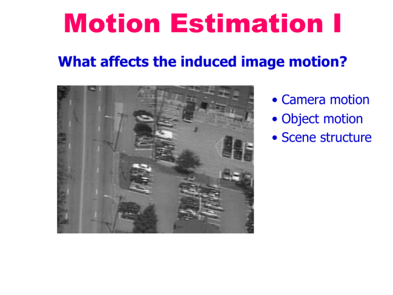
Motion Estimation I
What affects the induced image motion?
• Camera motion
• Object motion
• Scene structure
Example Flow Fields
• This lesson – estimation of general flow-fields
• Next lesson – constrained by global parametric transformations
The Aperture Problem
So how much information is there locally…?
The Aperture Problem
Not enough info in local regions
Copyright, 1996 © Dale Carnegie & Associates, Inc.
The Aperture Problem
Not enough info in local regions
Copyright, 1996 © Dale Carnegie & Associates, Inc.
The Aperture Problem
Copyright, 1996 © Dale Carnegie & Associates, Inc.
The Aperture Problem
Information is
propagated from
regions with high
certainty (e.g., corners)
to regions with low
certainty.
Copyright, 1996 © Dale Carnegie & Associates, Inc.
Such info propagation can cause
optical illusions…
Illusory corners
• Direct (intensity-based) Methods
1. Gradient-based (differential) methods
(Horn &Schunk, Lucase & Kanade)
2. Region-based methods
(Correlation, SSD, Normalized correlation)
• Feature-based Methods
Brightness Constancy Assumption
Image I
(taken at time t+1)
 x  u, y  v 
J x, y  
Image J
(taken at time t)
 x, y 
u, v 
I x  u , y  v 
The Brightness Constancy Constraint
Brightness Constancy Equation:
J ( x , y )  I ( x  u ( x , y ), y  v ( x , y ))
Linearizing (assuming small (u,v)):
J ( x, y )  I ( x, y )  I x ( x, y )  u ( x, y )  I y ( x, y )  v( x, y )
0  I x ( x, y )  u ( x, y )  I y ( x, y )  v( x, y )  I ( x, y )  J ( x, y )
 I x ( x, y )  u ( x, y )  I y ( x, y )  v( x, y )  I t ( x, y )
u ( x , y ) 
  I ( x, y )  
  I t ( x, y )
 v( x, y ) 
T
Observations:
* One equation, 2 unknowns
* A line constraint in (u,v) space.
𝐼𝑡
* Can recover “Normal-Flow” =
𝛻𝐼
(the component of the flow in the gradient direction)
Need additional constraints…
Horn and Schunk (1981)
Add global smoothness term
E 
 I
u  I yv  It    
2
x
 u
2
x
u
2
y
  v
2
x
v
( x, y)
(x,y)
Error in brightness
constancy equation
Minimize:
Smoothness error
Ec  Es
Solve by using calculus of variations
2
y

Horn and Schunk (1981)
Inherent problems:
* Smoothness assumption wrong at motion/depth
discontinuities
 over-smoothing of the flow field.
* How is Lambda determined…?
Lucas-Kanade (1984)
Assume a single displacement (u,v) for all pixels within a small
window (e.g., 5x5)
Geometrically -- Intersection of multiple line constraints
Algebraically --
E (u , v ) 
Minimize E(u,v):
 I
( x , y )W indow
( x , y )u  I y ( x , y )v  I t 
2
x
Lucas-Kanade (1984)
Minimize E(u,v):
E (u , v ) 
 I
( x , y )u  I y ( x , y )v  I t 
2
x
( x , y )W indow
Differentiating w.r.t u and v and equating to 0:
  I x2
 I x I y   u      I x I t 

2 

I
I
I
v
  x y
 y      I y I t 
  I  I 
T

U   I It
Solve for (u,v)
[ Repeat this process for each and every pixel in the image ]
Singularites
 I

  I x I y
2
x

I
I
 x y
2 
 I y 
Where in the image will this matrix be
invertible and where not…?
 Homework
Linearization approximation
 iterate & warp
estimate
update
Initial guess:
Estimate:
x0
x
Linearization approximation
 iterate & warp
estimate
update
Initial guess:
Estimate:
x0
x
Linearization approximation
 iterate & warp
estimate
update
Initial guess:
Estimate:
x0
x
Linearization approximation
 iterate & warp
x0
x
Revisiting the small motion assumption
Is this motion small enough?
Probably not—it’s much larger than one pixel (2nd order
terms dominate)
How might we solve this problem?
Coarse-to-Fine Estimation
Advantages: (i) Larger displacements. (ii) Speedup.
(iii) Information from multiple window sizes.
iterate
+
u
I x u  I y  v  It  0

u
refine
u=1.25 pixels

u=2.5 pixels
Δu
==> small u and v ...
u=5 pixels
image J
Pyramid of image J
u=10 pixels
image I
Pyramid of image I
Optical Flow Results
Optical Flow Results
Lucas-Kanade (1984)
Inherent problems:
* Still smoothes motion discontinuities
(but unlike Horn & Schunk, does not propagate error across the
entire image)
* Local singularities (due to the aperture problem)
• Maybe increase the aperture (window) size…?
• But no longer a single motion…
 Global parametric motion estimation – next week.
Motion Magnification
Wu, Rubinstein, Shih, Guttag, Durand, Freeman
“Eulerian Video Magnification for Revealing Subtle
Changes in the World”, SIGGRAPH 2012
Source video:
baby.mp4
Result: baby-iir-r1-0.4-r2-0.05-alpha-10-lambda_c-16-chromAtn-0.1.mp4
Paper + videos can be found on:
http://people.csail.mit.edu/mrub/vidmag
Motion Magnification
Could compute optical flow and magnify it
But…
very complicated (motions are almost invisible)
Alternatively:
𝐼𝑥 ∙ 𝑢 + 𝐼𝑦 ∙ 𝑣 = - 𝐼𝑡
𝐼𝑥 ∙ 𝑢•s + 𝐼𝑦 ∙ 𝑣•s = - 𝐼𝑡 •s
But holds only for small u•s and v•s
 apply coarse to fine to generate larger motions
Motion Magnification
What is 𝐼𝑡 •s equivalent to?
𝑰(𝒙, 𝒚)
𝒕 (time)
This is equivalent to keeping the same temporal frequencies,
but magnifying the amplitude (increase frequency coefficient).
 Can decide to do this selectively to specific temporal
frequencies (e.g., a range of frequencies of expected heart rates).
Motion Magnification
Wu, Rubinstein, Shih, Guttag, Durand, Freeman
“Eulerian Video Magnification for Revealing Subtle
Changes in the World”, SIGGRAPH 2012
Paper + videos can be found on:
http://people.csail.mit.edu/mrub/vidmag
A simplified version of this work
 the next programming exercise
• Exercise will be posted within a few days
• Meanwhile, please read SIGGRAPH’2012 paper