Geographic Information Processing
Raster Data Models
•
•
•
•
•
•
Data files
Metadata
Cell size
Cell alignment
Resampling
Smoothing
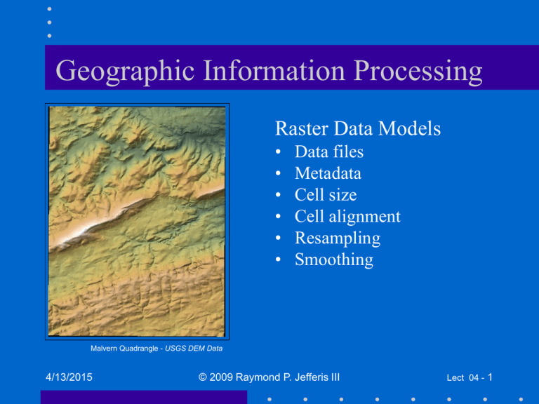
Malvern Quadrangle - USGS DEM Data
4/13/2015
© 2009 Raymond P. Jefferis III
Lect 04 - 1
Raster Data Files
•
•
•
•
Taken at regular intervals covering an area
The data cells are typically rectangular
The area is defined by its corner coordinates
The ordering of the data, within the file,
determines the spatial location of each cell
with respect to the corners
4/13/2015
© 2009 Raymond P. Jefferis III
Lect 04 - 2
USGS Digital Raster Graphics
Digital Geospatial Metadata
7.5-minute DRGs (scanned from older maps)
Projection: typically 1927 North American Datum
Available Scales:
1:12,000 (approx. 3.75' quadrangles)
1:24,000 (approx. 7.5' quadrangles - most common)
1:63,360 (approx. 15' quadrangles - abandoned)
1:100,000 (30' x 60' quadrangles)
1:250,000 (1˚ x 2˚ or 3 ˚ quadrangles)
Data supplied in TIFF format
4/13/2015
© 2009 Raymond P. Jefferis III
Lect 04 - 3
DRG Map Scale Comparison
Scale 1:24,000
4/13/2015
USGS
Scale 1:100,000
© 2009 Raymond P. Jefferis III
USGS
Lect 04 - 4
Digital Elevation Model (DEM) Data
• Arrays of regularly spaced elevations on
south-to-north profiles, ordered west-to-east
• 7.5', 30', or 1˚ sets, skewed from longitudes
• ASCII or binary elevation values
• Universal Transverse Mercator (UTM) or
geographic coordinate referenced
• Seamless version is National Elevation Data
(NED)
4/13/2015
© 2009 Raymond P. Jefferis III
Lect 04 - 5
DEM Availability
• Replaced by:
– National Elevation Dataset (NED) and,
– Spatial Data Transfer Standard (SDTS) data
• Download sites:
http://data.geocomm.com/dem/
http://edc2.usgs.gov/geodata/index.php
4/13/2015
© 2009 Raymond P. Jefferis III
Lect 04 - 6
National Elevation Dataset (NED)
•
•
•
•
•
•
Seamless raster dataset
Available from USGS
Elevations in meters
Resolution: 1arc-sec (approx. 30-meters)
Datum: North American Datum 1983
Metadata:
www.fgdc.gov
4/13/2015
© 2009 Raymond P. Jefferis III
Lect 04 - 7
DEM Scan Format
Standards for Digital Elevation models, Part 1, USGS
4/13/2015
© 2009 Raymond P. Jefferis III
Lect 04 - 8
DEM Standards
• Download for use with your datasets.
• Download site:
http://rockyweb.cr.usgs.gov/nmpstds/demstds.html
4/13/2015
© 2009 Raymond P. Jefferis III
Lect 04 - 9
Reading DEM Files in Mathematica®
ySR = Import[
"~/Desktop/DEMdata/PA/Malvern/1670812.dem.sdts.tgz",
{"SDTS",
"SpatialRange"}]
yER = Import[
"~/Desktop/DEMdata/PA/Malvern/1670812.dem.sdts.tgz",
{"SDTS",
"ElevationRange"}]
•Spatial range result [meters]:
{{446655, 457365}, {4427685, 4441605}}
•Elevation range result [feet]:
{0, 720}
4/13/2015
© 2009 Raymond P. Jefferis III
Lect 04 - 10
Extracting Data Parameters
dims = Dimensions[yDat]; (* get metadata *)
nbase = dims[[1]];(* Skip *)
nrows = dims[[2]];(*number of data rows -> 465 *)
ncols = dims[[3]]; (* number of data columns -> 358 *)
minval = yER[[1]]; (* minimum altitude, feet *)
maxval = yER[[2]]; (* maximmum altitude, feet *)
4/13/2015
© 2009 Raymond P. Jefferis III
Lect 04 - 11
Reading DEM File in Mathematica®
Import data:
yDat = Import[
"~/Desktop/DEMdata/PA/Malvern/1670812.dem.sdts.tgz", {"SDTS",
"Data"}];
Look at the elevation data of one row:
y = yDat[[1, 465]]
The result is:
{0, 0, 0, 418, 408, 402, 394, 387, 375, 372, 386, 394, 393, 386, 378, 375, ¥
372, 373, 373, 372, 371, 369, 361, 354, 348, 350, 350, 350, 350, 353, 354, ¥
357, 358, 361, 364, 366, 368, 369, 379, 397, 407, 397, 388, 376, 367, 359, ¥
352, 345, 340, 334, 329, 323, 316, 310, 306, 304, 304, 304, 305, 306, 308, ¥
310, 312, 315, 320, 326, 330, 334, 337, 338, 338, 337, 334, 327, 322, 316, ¥
304, 298, 292, 288, 286, 285, 285, 286, 290, 294, 302, 313, 321, 334, 350, ¥
381, 400, 442, 486, 497, 483, 461, 449, 0, 0, 0, 0, 0, 0, 0, 0, 0, 0, 0, 0, ¥
0, 0, 0, 0, 0, 0, 0, 0, 0, 0, 0, 0, 0, 0, 0, 0, 0, 0, 0, 0, 0, 0, 0, 0, 0, 0, ¥
0, 0, 0, 0, 0, 0, 0, 0, 0, 0, 0, 0, 0, 0, 0, 0, 0, 0, 0, 0, 0, 0, 0, 0, 0, 0, ¥
0, 0, 0, 0, 0, 0, 0, 0, 0, 0, 0, 0, 0, 0, 0, 0, 0, 0, 0, 0, 0, 0, 0, 0, 0, 0, ¥
0, 0, 0, 0, 0, 0, 0, 0, 0, 0, 0, 0, 0, 0, 0, 0, 0, 0, 0, 0, 0, 0, 0, 0, 0, 0, ¥
0, 0, 0, 0, 0, 0, 0, 0, 0, 0, 0, 0, 0, 0, 0, 0, 0, 0, 0, 0, 0, 0, 0, 0, 0, 0, ¥
0, 0, 0, 0, 0, 0, 0, 0, 0, 0, 0, 0, 0, 0, 0, 0, 0, 0, 0, 0, 0, 0, 0, 0, 0, 0, ¥
0, 0, 0, 0, 0, 0, 0, 0, 0, 0, 0, 0, 0, 0, 0, 0, 0, 0, 0, 0, 0, 0, 0, 0, 0, 0, ¥
0, 0, 0, 0, 0, 0, 0, 0, 0, 0, 0, 0, 0, 0, 0, 0, 0, 0, 0, 0, 0, 0, 0, 0, 0, 0, ¥
0, 0, 0, 0, 0, 0, 0, 0, 0, 0, 0, 0, 0, 0, 0, 0, 0, 0, 0, 0, 0, 0, 0, 0, 0, 0, ¥
0, 0, 0, 0, 0, 0, 0, 0, 0, 0, 0, 0, 0}
4/13/2015
© 2009 Raymond P. Jefferis III
Lect 04 - 12
Viewing DEM File in Mathematica®
yGrf = Import[
"~/Desktop/DEMdata/PA/Malvern/1670812.dem.sdts.tgz",
"SDTS"];
Notes:
• Raster skew, leading to
missing data, at edges
of quadrangle
• Older file data
• Image slightly blurred
4/13/2015
© 2009 Raymond P. Jefferis III
Lect 04 - 13
Plotting Data in Mathematica®
elev = Table[yDat[[1, r, c]], {r, 1, nrows, 1}, {c, 1,
ncols, 1}];
ReliefPlot[elev, ColorFunction -> "GreenBrownTerrain"]
Notes:
• First step makes table of
sampled data, which can be
used for further processing
• Second step plots it
• Image is crisp
• Pixels approx. 30 x 30 meters
4/13/2015
© 2009 Raymond P. Jefferis III
Lect 04 - 14
Calculation, from Lecture #2
At 40˚ North latitude, 76˚ West longitude, a square of 7.5´
will have the planar dimensions:
North_Distance = 13.8793 km
463 30 meter cells
East_Distance = 10.6742 km
356 30 meter cells
4/13/2015
© 2009 Raymond P. Jefferis III
Lect 04 - 15
Calculation, from File Data
At 40˚ North latitude, 75.625˚ West longitude, a
square of 7.5´ will have the planar dimensions:
North_Distance = 13.920 km
464 30 meter cells
East_Distance = 10.710 km
357 30 meter cells
Note: There is one more row and column in the file,
so that the data go all the way to the edges.
4/13/2015
© 2009 Raymond P. Jefferis III
Lect 04 - 16
Metadata
•
•
•
•
Data about the data
Gives resolution, units, datum, etc.
Needed for interpreting data
Data storage format given in specifications
located separately
4/13/2015
© 2009 Raymond P. Jefferis III
Lect 04 - 17
Selected Metadata
•
•
•
•
•
•
•
•
•
•
•
•
•
•
•
ITEM_TYPE: SDTS DEM - 7.5X7.5 GRID
CELL_NAME: Malvern
X_RESOLUTION: 30
Y_RESOLUTION: 30
XY_UNITS: Meter
Z_RESOLUTION: 1.000
Z_UNITS: Foot
HORIZONTAL_DATUM: North American Datum of 1927
PROJECTION: Transverse Mercator
MIN_ELEVATION: 105
MAX_ELEVATION: 720
NORTH_LATITUDE: 40.125000
SOUTH_LATITUDE: 40.000000
WEST_LONGITUDE: -75.625000
EAST_LONGITUDE: -75.500000
4/13/2015
© 2009 Raymond P. Jefferis III
Lect 04 - 18
Calibration of Data
• Locate known landmark or benchmark
feature coordinates
• Proportion pixel count to find data
• Draw mark at location on figure
• Replot data with modified feature
• Check with USGS topographic map
4/13/2015
© 2009 Raymond P. Jefferis III
Lect 04 - 19
Example
Antenna known to be on top of ridge:
(* Bacton Hills Antenna Location *)
antlat = 40.058327; [North]
antlon = 75.598366; [West]
Define quadrangle corners:
(* Malvern Quadrangle Corners*)
nelat = 40.125;
nelon = 75.500;
swlat = 40.000;
swlon = 75.625;
4/13/2015
© 2009 Raymond P. Jefferis III
Lect 04 - 20
Example (continued)
Locate {x,y} data pixel of feature:
(* Proportion Pixels from SW Corner*)
latpt = Round[nrows*((antlat swlat))/(nelat - swlat)];
lonpt = Round[ncols*((swlon antlon))/(swlon - nelon)];
4/13/2015
© 2009 Raymond P. Jefferis III
Lect 04 - 21
Example (continued)
• Draw crosshairs (set height to sea level!)
(* Draw Crosshairs *)
yDat[[1, latpt, lonpt]] = 0;
yDat[[1, latpt + 1, lonpt]] =
yDat[[1, latpt + 2, lonpt]] =
yDat[[1, latpt - 1, lonpt]] =
yDat[[1, latpt - 2, lonpt]] =
yDat[[1, latpt, lonpt + 1]] =
yDat[[1, latpt, lonpt + 2]] =
yDat[[1, latpt, lonpt - 1]] =
yDat[[1, latpt, lonpt - 2]] =
4/13/2015
0;
0;
0;
0;
0;
0;
0;
0;
© 2009 Raymond P. Jefferis III
Lect 04 - 22
Example (plotted result)
==>
4/13/2015
• Crosshairs on
ridgeline
• Location correct
• Plot oriented
correctly
• Find corresponding
Mathematica®
notebook in Models
file as:
MalvernBactonTest
© 2009 Raymond P. Jefferis III
Lect 04 - 23
DTED Data File Format
•
•
•
•
(1) User Header Label (UHL: 80 bytes)
(2) Data Set Identification Record (DSI: 648 bytes)
(3) Accuracy Record (ACC: 2700 bytes)*
(4) Data Records (3601 records at 7214
10642, 17856,etc. bytes/record)**
1
81
729
3429,
** The number of records is a function of the latitude. A count of 3601 is
for cells between latitudes S50 and N50 degrees. Missing elevations
are filled with 1 bits. Elevations are two-byte integers, high order first,
and negatives are signed magnitude.
4/13/2015
© 2009 Raymond P. Jefferis III
Lect 04 - 24
Reading DTED File
See MalvernDTED notebook in Models
directory
4/13/2015
© 2009 Raymond P. Jefferis III
Lect 04 - 25
Reading DTED File Header
(* Define and read in data for DTED data set *)
Array[d, 2000, 2000];
s=
OpenRead["~/Desktop/DTEDdata/w076n40.dt2"];
(*Read Header information *)
uhl = ReadList[s, Character, 80];
dsi = ReadList[s, Character, 648];
acc = ReadList[s, Character, 2700];
4/13/2015
© 2009 Raymond P. Jefferis III
Lect 04 - 26
Reading DTED File
(* Read the data and convert to signed integer format *)
(* Offset to Malvern Quadrangle *)
mm = 1350;
ll = 450; (* Width in rows *)
For[j = mm, j < mm + ll, j++, {
(* Read record header *)
SetStreamPosition[s, 3428 + j*7214];
bh = Read[s, Byte];
bl = Read[s, Byte];
c1 = 256*Read[s, Byte] + Read[s, Byte];
c2 = 256*Read[s, Byte] + Read[s, Byte];
c3 = 256*Read[s, Byte] + Read[s, Byte];
rr = 0;(* Read data column *)
For[i = 0, i < ll + 1, i++,{
d[i, j - mm] = 256*Read[s, Byte] + Read[s, Byte]; }]
}]
Close[s];
4/13/2015
© 2009 Raymond P. Jefferis III
Lect 04 - 27
Plotted Result
Notes:
(Malvern Quadrangle)
•
•
•
•
4/13/2015
High resolution [10 meters]
Processing to Level 2
Data to edges
One-column overlap
at edges (451 columns)
© 2009 Raymond P. Jefferis III
Lect 04 - 28
Calibration
• Mark a known feature on plotted result and
compare with its known location
–
–
–
–
Mountaintop
Stream intersection
Lake
Quarry
4/13/2015
© 2009 Raymond P. Jefferis III
Lect 04 - 29
Calibration
Notes:
• Crosshairs at
Bacton Hill
antenna site.
• Location correct
4/13/2015
© 2009 Raymond P. Jefferis III
Lect 04 - 30
SRTM Files [.HGT ]
• Heights are signed two byte integers.
• The bytes are in Motorola "big-endian" order
with the most significant byte first.
• Heights are in meters referenced to the
WGS84/EGM96 geoid. Data voids are
assigned the value -32768.
• SRTM1 files contain 3601 lines of 3601
samples each, with edge overlap.
• IMPORTANT! - NW-to-SE order
4/13/2015
© 2009 Raymond P. Jefferis III
Lect 04 - 31
Reading SRTM1 Files
See hgt2Test notebook in Models file
Note: Data are in binary bytes, stored as rows
(not columns), read from NW to SE
(software will reverse).
4/13/2015
© 2009 Raymond P. Jefferis III
Lect 04 - 32
Reading SRTM1 Files [.HGT]
Array[d, 3601, 3601];
s = OpenRead["~/Desktop/N40W076.hgt",
BinaryFormat -> True];
nn = 1350;
nrows = 450;
ncols = 450;
For[j = 0, j < nrows + 1, j++,
SetStreamPosition[s, nn*2 + 7202*(3600 - j)];
For[i = 0, i < ncols + 1, i++,
d[i, j] =
256*BinaryRead[s, "UnsignedInteger8"] +
BinaryRead[s, "UnsignedInteger8"] ]; ];
(* Close data file *)
Close[s];
4/13/2015
© 2009 Raymond P. Jefferis III
Lect 04 - 33
Results
Notes:
• High resolution
image
• Processed to
remove voids
• No gaps at edges
4/13/2015
© 2009 Raymond P. Jefferis III
Lect 04 - 34
Resampling
• Result is new image derived from original
• Each pixel is weighted sum of surrounding
pixels
• Principal methods
– Straight sampling (to reduce raster points)
– Bilinear interpolation (for off-grid points)
– Cubic convolution (for regular raster points)
4/13/2015
© 2009 Raymond P. Jefferis III
Lect 04 - 35
Simple Resampling
•
•
•
•
Pick every nth pixel
No pixel averaging
Result is fewer pixels but no noise reduction
Images look “jaggy”
4/13/2015
© 2009 Raymond P. Jefferis III
Lect 04 - 36
Simple Resampling [5:1]
sampledelev =
Table[d[r + rowmin, c + colmin], {r,
0, nrows, 5}, {c, 0, ncols, 5}];
ReliefPlot[sampledelev, AspectRatio ->
13.8793/10.6742,
ColorFunction -> "GreenBrownTerrain"]
Note: Pixel aspect ratio is defined from
calculation results of Slides 15 and 16.
4/13/2015
© 2009 Raymond P. Jefferis III
Lect 04 - 37
Resampled 2:1 and 5:1 Quadrangles
4/13/2015
© 2009 Raymond P. Jefferis III
Lect 04 - 38
Re-sampling with Smoothing
• Pick every nth pixel
• Form new value from weighted sum of this
pixel and its surrounding ones.
• Result: fewer pixels, some noise reduction
• Images look “jaggy”
4/13/2015
© 2009 Raymond P. Jefferis III
Lect 04 - 39
Resulting Resampled Data
• Fewer pixels per square ground area
• More area can be covered
• Note: SRTM3 data could be used instead
– 30 x 30 meter (approx.) pixels
– Each pixel averages nine (9) SRTM1 pixels
– Averaging improves statistical accuracy
4/13/2015
© 2009 Raymond P. Jefferis III
Lect 04 - 40
Bilinear Interpolation
d1 1
d2 1
d3 1
d4 1
d5 1
d1 2
d22
d32
d42
d5 2
d1 3
d23
d33
d43
d5 3
d1 4
d24
d34
d44
d5 4
d1 5
d2 5
d3 5
d4 5
d5 5
Portion of data to be
resampled to give value of
data at new point, d33
• Pixel d33 can be off-grid, others are
nearby points for extrapolation
• Pixel d33 is to be distance-weighted sum
of pixels d22, d24, d42, and d44
• x-distance is (x33/x32)*(x34-x32)
• y-distance is (y33/y43)*(y23-y43)
4/13/2015
© 2009 Raymond P. Jefferis III
Lect 04 - 41
Convolution
• Value of raster point determined from weighted
sum of others
• Simple averaging includes the 8 closest pixels,
weighted by distance from the center pixel
• Cubic convolution uses the 16 closest pixels
• Convolution kernel needed
• Resulting values should be normalized by the sum
of weights to retain proper scale
4/13/2015
© 2009 Raymond P. Jefferis III
Lect 04 - 42
Averaging Convolution Kernel
0 .7 0 7
1
0 .7 0 7
1
1
1
0 .7 0 7
1
/7 .8 2 8
0 .7 0 7
Note: Cells are weighted by distance from
the center cell, and the array of weights is
then normalized by the sum of weights.
4/13/2015
© 2009 Raymond P. Jefferis III
Lect 04 - 43
Results
• Raw data represent 10 x 10 meter areas
• Averaged data represent 30 x 30 meter areas
• Raw data images are sharp; averaged data
appear blurry.
• Raw data contours are jaggy; contours of
averaged data are smoother.
• Images follow:
4/13/2015
© 2009 Raymond P. Jefferis III
Lect 04 - 44
Raw and Averaged Data Images
Raw Data - Malvern
4/13/2015
Averaged Data
© 2009 Raymond P. Jefferis III
Lect 04 - 45
Raw and Averaged Contours
Raw Data - Malvern
4/13/2015
Averaged Data
© 2009 Raymond P. Jefferis III
Lect 04 - 46
Contours - Summary
• Smoothing important for contour maps
• Convolution is effective for processing
4/13/2015
© 2009 Raymond P. Jefferis III
Lect 04 - 47
Questions?
4/13/2015
© 2009 Raymond P. Jefferis III
Lect 04 - 48