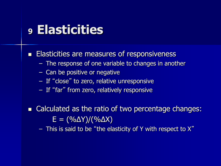
9
Elasticities

Elasticities are measures of responsiveness
–
–
–
–

The response of one variable to changes in another
Can be positive or negative
If “close” to zero, relative unresponsive
If “far” from zero, relatively responsive
Calculated as the ratio of two percentage changes:
E = (%∆Y)/(%∆X)
– This is said to be “the elasticity of Y with respect to X”
Consider this relationship

The elasticity of grades
with respect to
Study Time/week
time spent studying
– Likely positive
– Ε = (%∆G)/(%∆S) > 0
– If E > 1, we say “elastic”
(relatively responsive)
– If E < 1, we say “inelastic”
(relatively unresponsive)
0
Grade
Another example

The elasticity of grades
with respect to
alcohol consumption
Alcohol Consumption/week
– Likely negative
– E = (%∆G)/(%∆A) < 0
– If |E| >1, we say “elastic”
(relatively responsive)
– If |E| < 1, we say “inelastic”
(relatively unresponsive)
0
Grades
The (own) Price Elasticity of Demand

Measures the responsiveness of quantity demanded
to changes in the price of the good itself
– Defined thus:
 ε = [(%∆in quantity demanded)/(%∆ in price)]
 Or ε = [(%∆Qd)/(%∆P)]

Note that ε must be negative (Law of Demand)

Sometimes convenient to refer to the absolute
value |ε| so we can ignore the negative sign
Examples of demand elasticities
Suppose a 10% rise in the price of a good causes a
20% reduction in the quantity demanded in a
measured time period
ε = -20%/+10% = -2
Suppose a 15% decline in the price of a good causes
a 10% increase quantity demanded in a measured
time period
ε = +10%/-15% = -0.67
Categories of demand elasticities
“Elastic” demand

Elastic demand
– elasticity > 1
Price
– Qd relatively responsive to price
Demand
– Price change leads to spending
change in opposite direction
– Thus,
 Higher price → lower spending
 Lower price → higher spending
Q/time
When is a good likely to
have sensitive elasticity?
If a product is not unique so it has many close
substitutes and consumers know about the
alternatives.
When buyers’ expenditures are a large part of
their income so they shop more carefully—
buying a home.
The product is an input in production that is
price sensitive, so the producer will keep
close watch on input prices.
Demand elasticity . . .
“Inelastic” demand

Inelastic demand
– elasticity < 1
Price
– Qd relatively unresponsive to price
– Price change leads to spending
change in same direction
– Thus,
 Higher price → higher spending
 Lower price → lower spending
Demand
Q/time
When is elasticity likely
to be less sensitive?
When comparisons to substitutes is difficult. Examples:
Door-to-door sales. Complex products that are hard
to compare.
When consumers pay only a fraction of the cost. Ex.:
When insurance covers most of the bill.
When the cost of switching would be high. Example:
When the user has developed expertise in using a
product (software).
When a product is used with another product that the
consumer uses.
Example: Ink cartridges in printers.
Some uses of demand elasticities



More Accurate Pricing
– Use of UPC bar codes to aid in pricing products
(e.g., Wal-Mart and other retailers data)
Trying to Maximize Profits
– A higher price is no guarantee of higher revenue
(will study below)
Plan ahead
– If you know about future events — plan more
precisely (hotels and conventions)
No close substitutes?
SCI, the largest firm in the U.S. funeral business, with
14% of total industry revenue, increased its average
revenue per service (its product price) by 9% in one
year. The number of funeral services fell by 5.8%.
The price elasticity of demand for its services is –
(-5.8/9) = 0.64. Its price and quantity demanded
suggest that its demand is inelastic—and we know from
this calculation that its total revenue increased from
these services increases.
Was the price increase sensible?
Real World Elasticities
(all negative numbers)
Product or Service
Lamb
Bread
Coffee
Tires
Auto Repairs
Theatre & Opera
Movies
Foreign Travel by U.S. Residents
Public Transportation
Electricity
Jewelry & Watches
Alcohol and Tobacco
Recreation
Estimated Elasticity
Short Run
Long Run
2.65
0.15
0.16
0.8
1.4
0.2
0.9
0.1
0.6
0.1
0.4
0.3
1.1
---1.2
2.4
0.3
3.7
1.8
1.2
1.8
0.6
0.9
3.5
Example







ESPN football videogame:
2003 price: $40
2004 price: $20 (50% decrease)
2003 Qd: 400,000
2004 Qd: 2.7 million (575% increase)
E = 575%/50% = 11.5
Note: major competitor, Madden football,
did not change price; its sales rose less than
10% from 2003 to 2004
How a market changes
when prices change
Hong Kong had 80% tariff on wine, so
high wine prices.
2008: tariff abolished; retail prices fell 3050%.
Sales rose: 34% in ’09; 73% in ‘10 and
40% in ‘11.
Elasticity appears near 1.
What else changed?
Little impact in restaurants since they
have large markup already.
Sale increase was at stores.
Expanded volume meant increase need
for warehouse space, HK became largest
wine auction site in world in ‘11 (quarter
billion in auction sales).
Wine expos. Greater employment.
Smuggling ended.
Cross-price elasticities

Cross-price elasticity of demand
– Measure of responsiveness of demand to
changes in prices of substitutes and
complements:
(%∆ Dx) / (%∆ Py)
– If positive, goods are substitutes, by
definition
– If negative, goods are complements, by
definition
Estimates of Cross Elasticities

These are estimates of cross elasticities of various
goods (goods that are substitutes) in the U.S.:
Electricity and natural gas
Beef and Pork
Natural gas and fuel oil
Margarine and butter
0.20 (weak substitutes)
0.20
0.44
0.81 (strong substitutes)
Income Elasticity of Demand
– Measure of responsiveness of demand to changes
in income: (%∆ Dx) / (%∆ l)
– If positive, good is normal (>1, superior)
– If negative, good is inferior, by definition
Recession in U.S.—Incomes down 4%:
‘08-09—Budweiser down 7.4%; Busch up 5.3%
Saks down 26%; Wal-Mart up 3.5%
2010: Concert Ticket Sales fell 15% in U.S.
Lowe’s: home repair projects over $500 way down.
Estimates of Income Elasticities
Estimates of income elasticities from different studies
in the U.S.:
Flour
-0.36 (inferior good)
Margarine
-0.20 (inferior good)
Milk and cream
0.07 (little change)
Beef
0.51 to 1.05
Apples
1.32
Dental Services
1.41 (highly responsive to
Restaurant meals
1.48 income increases)
Personal air travel 1.8

Elasticity

A study of gasoline sales found that
price elasticity for regular gasoline was
-0.6; for premium gasoline was -0.3.
Why the difference?