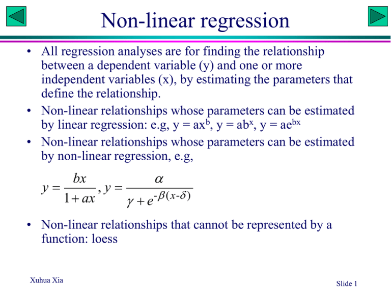
Non-linear regression
• All regression analyses are for finding the relationship
between a dependent variable (y) and one or more
independent variables (x), by estimating the parameters that
define the relationship.
• Non-linear relationships whose parameters can be estimated
by linear regression: e.g, y = axb, y = abx, y = aebx
• Non-linear relationships whose parameters can be estimated
by non-linear regression, e.g,
bx

y
,y
1  ax
  e-  ( x - )
• Non-linear relationships that cannot be represented by a
function: loess
Xuhua Xia
Slide 1
Growth curve of E. coli
• A researcher wishes to estimate the growth curve of
E. coli. He put a very small number of E. coli cells
into a large flask with rich growth medium, and take
samples every half an hour to estimate the density
(n/L).
• 14 data points over 7 hours were obtained.
• What is the instantaneous rate of growth (r). What is
the initial density (N0)?
• As the flask is very large, he assumed that the growth
should be exponential, i.e., y = a·ebx (Which
parameter correspond to r and which to N0?)
Xuhua Xia
Slide 3
SAS Program
/* Fictitious data */
data Ecoli;
Input Density @@;
Time = _N_;
lnD = log(Density);
datalines;
20.023 39.833 80.571 161.102 317.923 635.672 1284.544 2569.430
5082.654 10220.777 20673.873 40591.439 81374.642 163963.873
;
proc reg;
This statement is necessary, otherwise Density
var Density lnD Time;
will be an unknown variable for the reg
model lnD = Time;
procedure and the plot statement will fail.
plot Density*Time/ symbol='.';
plot lnD*Time/ symbol='.';
Run, and ask students to compute
run;
parameters a and b from regression
output. What is the initial density?
Xuhua Xia
Slide 4
Body weight of wild elephant
• A researcher wishes to estimate the body weight of wild
elephants.
• He measured the body weight of 13 captured elephants of
different sizes as well as a number of predictor variables, such
as leg length, trunk length, etc. Through stepwise regression,
he found that the inter-leg distance (shown in figiure) is the
best predictor of body weight.
• He learned from his former biology professor that the
allometric law governing the body weight (W) and the length
of a body part (L) states that
W = aLb
• Use linear regression to find
parameters a and b.
Xuhua Xia
Slide 5
SAS Program
/*Fitcitious data */
data Elephant;
Input L W @@;
lnL = log(L);
lnW = log(W);
datalines;
0.3 1.657 0.4 2.500 0.5 4.680 0.6 7.075 0.7 10.070
0.8 11.988 0.9 14.836 1 18.318 1.1 23.496 1.2 27.897
1.3 36.796 1.4 44.611 1.5 50.183
;
proc reg;
Run and ask students to
var L W lnL lnW;
calculate the parameters a
model lnW = lnL;
and b.
plot W*L/ symbol='.';
plot lnW*lnL/ symbol='.';
run;
Xuhua Xia
Slide 6
DNA and protein gel electrophoresis
• How to estimate the molecular
mass of a protein?
– A ladder: proteins with known
molecular mass
– Deriving a calibration curve
relating molecular mass (M) to
migration distance (D): D =
F(M)
– Measure D and obtain M
• The calibration curve is
obtained by fitting a regression
model
Xuhua Xia
Slide 7
Protein molecular mass
• The equation appears to describe the
relationship between D and M quite well.
This relationship is better than some
published relationships, e.g.,
D = a – b ln(M)
• The data are my measurement of D and
M for a subset of secreted proteins from
the gastric pathogen Helicobacter pylori
(Bumann et al., 2002).
• Write a SAS program to use the data to
find parameters a and b
D  ae
bM
Mass
D
5
14.5
10
12.6
20
9.4
30
7.1
40
5.3
50
3.9
60
3.05
70
2.3
80
1.75
Bumann, D., Aksu, S., Wendland, M., Janek, K., Zimny-Arndt, U., Sabarth, N., Meyer, T.F., and
Jungblut, P.R., 2002, Proteome analysis of secreted proteins of the gastric pathogen Helicobacter pylori.
Infect. Immun. 70: 3396-3403.
Xuhua Xia
Slide 8
Area and Radius
What is the functional relationship
between the area and the radius?
Xuhua Xia
Toxicity study: pesticide
100
90
Percentage killed
80
70
60
50
40
30
20
10
0
25
30
35
40
45
50
55
60
65
70
Dosage
What transformation to use?
Xuhua Xia
Slide 10
Probit and probit transformation
• Probit has two names/definitions, both
associated with standard normal
distribution:
– the inverse cumulative distribution
function (CDF)
– quantile function
0.9
0.8
0.7
0.6
CDF
• CDF is denoted (z), which is a
continuous, monotone increasing
sigmoid function in the range of (0,1),
e.g.,
(z) = p
(-1.96) = 0.025 = 1 - (1.96)
• The probit function gives the 'inverse'
computation, formally denoted -1(p),
i.e.,
probit(p) = -1(p)
probit(0.025) = -1.96 = -probit(0.975)
• [probit(p)] = p, and probit[(z)] = z.
1
0.5
0.4
0.3
0.2
0.1
0
-2.5
-1.5
-0.5
0.5
1.5
z
Xuhua Xia
Slide 11
SAS program
Data Pesticide;
Input Dosage Percent @@;
Why
NuProbit = probit(Percent/100);
Cards;
27 0.90 28 1.39 31 2.40 31 2.49 35 6.42 36 7.78 37 9.16
38 10.21 38 11.71 40 16.24 41 16.90 43 22.94 44 27.35
44 27.45 44 28.14 45 28.97 45 29.96 45 30.50 46 34.30
46 35.39 46 35.65 47 37.55 47 38.46 48 40.97 49 44.37
49 45.71 49 46.66 49 47.38 50 49.86 50 52.26 51 55.12
51 56.12 52 57.68 52 59.99 52 60.30 53 60.51 53 61.82
53 62.00 53 62.92 54 66.06 54 67.14 55 70.58 55 71.57
56 74.11 56 74.12 57 76.77 57 77.01 58 78.56 58 79.01
59 83.53 60 83.96 60 84.40 61 87.95 62 88.74 63 91.13
64 92.64 64 92.67 66 95.49 68 97.00 69 97.15
;
Proc reg;
Model Percent = Dosage / R CLM alpha = 0.01 CLI;
Plot Percent*Dosage / symbol = '.';
Model NuProbit = Dosage / R CLM alpha = 0.01 CLI;
Plot NuProbit*Dosage / symbol = '.';
run;
Xuhua Xia
divide Percent by 100?
Run and
explain
CLM: CL of mean
CLI: CL of individual observation
Graphic contrast
between the original
and the transformed DV
Slide 12
Non-linear regression
• In rapidly replicating unicellular eukaryotes such as
the yeast, highly expressed intron-containing genes
requires more efficient splicing sites than lowly
expressed genes.
• Natural selection will operate on the mutations at the
slicing sites to optimize splicing efficiency.
• Designate splicing efficiency as SE and gene
expression as GE.
• Certain biochemical reasoning suggests that SE and
GE will follow the following relationships:

   GE   GE 2 if GE  GE0 

E[ SE | GE ]  

if GE  GE0 

c

Xuhua Xia
GE
SE
1
0.46
2
0.47
3
0.57
4
0.61
5
0.62
6
0.68
7
0.69
8
0.78
9
0.7
10
0.74
11
0.77
12
0.78
13
0.74
13
0.8
15
0.8
16
0.78
Slide 14
Guess initial values
   GE   GE 2 if GE  GE0 
E[ SE | GE ]  

c
if
GE

GE
0

0.85
When GE=0 then SE = , so   0.4
0.8
When GE increases from 2 to 8, SE
increases from 0.47 to 0.75, so
  (0.75-0.47)/(8-2)  0.047
0.75
0.7
With   0.4 and   0.047, then SE for
GE = 12 should be 0.4+0.04712 =
0.96, but the actual SE is only about
0.77. This must be due to the quadratic
term GE2, i.e.,
SE
0.65
0.6
0.55
0.5
(0.77 - 0.96) =  122, so
0.45
  - 0.002
0.4
0
2
4
6
8
10
12
14
16
GE
Xuhua Xia
Slide 15
A few more twists

   GE   GE 2 if GE  GE0 

E[ SE | GE ]  

if GE  GE0 

c

The continuity condition requires that
E[SE | GE0 ]     GE0   GE02
The smoothness condition requires that
E[ SE | GE0 ]
   2 GE0  0
GE0
The two conditions implies that
GE0 
c 

2
  GE0   GE02
Xuhua Xia
2
 
4
Slide 16
SAS program
/* Fictitious data */
data Intron;
input SE GE @@;
datalines;
.46 1 .47 2 .57 3 .61 4 .62 5 .68 6 .69 7 .78 8 .70 9
.74 10 .77 11 .78 12 .74 13 .80 13 .80 15 .78 16
;
title 'Quadratic Model with Plateau';
proc nlin data=Intron;
Initial guestimates
parms alpha=.4 beta=.047 gamma=-.002;
GE0 = -.5*beta / gamma;
if (GE < GE0) then Y = alpha + beta*GE + gamma*GE*GE;
else Y = alpha + beta*GE0 + gamma*GE0*GE0;
A conditional statement
model SE = Y;
needed to model the two
if _obs_ =1 and _iter_ =. then do;
segments
plateau =alpha + beta*GE0 + gamma*GE0*GE0;
put / GE0= plateau= ;
Write out GE0 and plateau (which could
end;
be computed from the estimated , , and
output out=b predicted=SEp;
. However, the output of these parameters
run;
Xuhua Xia
computes predicted values
for plotting and saves them
to data set b
contain rounding errors.
Run and explain
Slide 17
Plot
proc sgplot data=b noautolegend;
yaxis label='Observed or Predicted';
refline 0.7775 / axis=y label="Plateau" labelpos=min;
refline 12.7476 / axis=x label="GE0" labelpos=min;
scatter y=SE x=GE;
series y=SEp x=GE;
run;
Xuhua Xia
Slide 18
Fitting another function
/* Fictitious data */
data Intron;
input SE GE @@;
datalines;
.46 1 .47 2 .57 3 .61 4 .62 5 .68 6 .69 7 .78 8 .70 9
.74 10 .77 11 .78 12 .74 13 .80 13 .80 15 .78 16
;
title 'Quadratic Model with Plateau';
proc nlin data=Intron;
parms alpha=.4 beta=.8 gamma=1;
model SE = (alpha+beta*GE)/(1+gamma*GE);
output out=b predicted=SEp;
SE 
run;
proc sgplot data=b noautolegend;
yaxis label='Observed or Predicted';
scatter y=SE x=GE;
series y=SEp x=GE;
run;
   GE
1   GE
Run and explain the output
Xuhua Xia
Slide 19
Plot output
Xuhua Xia
Slide 20
Robust regression
• LOWESS: robust local regression between Y and X, with
linear fitting
• LOESS: robust local regression between Y and one or more
Xs, with linear or quadratic fitting
• Used with relations that cannot be expressed in functional
forms
• SAS: proc loess
• Data:
– Data set 1: monthly averaged atmospheric pressure differences
between Easter Island and Darwin, Australia for a period of 168
months (NIST, 1998), suspected to exhibit 12-month (annual), 42month (El Nino), and 25-month (Southern Oscillation) cycles (From
Robert Cohen of SAS Institute)
– Data set 2: Two-channel microarray data. Background correction and
two-channel loess normalization (from Wudu).
Xuhua Xia
Slide 21
SmoothingParameter=0.2
Pressure
18
17
16
15
14
13
12
11
10
9
8
7
6
5
4
3
2
1
0
0
10
20
30
40
50
60
70
80
90
Month
100
110
120
130
140
150
160
170
SmoothingParameter=0.05
Pressure
18
17
16
15
14
13
12
11
10
9
8
7
6
5
4
3
2
1
0
0
10
20
30
40
50
60
70
80
90
Month
100
110
120
130
140
150
160
170
Step 1: characterize the most obvious
trend.
data ENSO;
input Pressure @@;
Month=_N_;
datalines;
12.9 11.3 10.6 11.2 10.9 7.5 7.7 11.7 12.9 14.3 10.9 13.7 17.1 14.0 15.3 8.5
5.7 5.5 7.6 8.6 7.3 7.6 12.7 11.0 12.7 12.9 13.0 10.9 10.4 10.2 8.0 10.9
13.6 10.5 9.2 12.4 12.7 13.3 10.1 7.8 4.8 3.0 2.5 6.3 9.7 11.6 8.6 12.4
10.5 13.3 10.4 8.1 3.7 10.7 5.1 10.4 10.9 11.7 11.4 13.7 14.1 14.0 12.5 6.3
9.6 11.7 5.0 10.8 12.7 10.8 11.8 12.6 15.7 12.6 14.8 7.8 7.1 11.2 8.1 6.4
5.2 12.0 10.2 12.7 10.2 14.7 12.2 7.1 5.7 6.7 3.9 8.5 8.3 10.8 16.7 12.6
12.5 12.5 9.8 7.2 4.1 10.6 10.1 10.1 11.9 13.6 16.3 17.6 15.5 16.0 15.2 11.2
14.3 14.5 8.5 12.0 12.7 11.3 14.5 15.1 10.4 11.5 13.4 7.5 0.6 0.3 5.5 5.0
4.6 8.2 9.9 9.2 12.5 10.9 9.9 8.9 7.6 9.5 8.4 10.7 13.6 13.7 13.7 16.5
16.8 17.1 15.4 9.5 6.1 10.1 9.3 5.3 11.2 16.6 15.6 12.0 11.5 8.6 13.8 8.7
8.6 8.6 8.7 12.8 13.2 14.0 13.4 14.8
;
ods output OutputStatistics=ENSOstats FitSummary=ENSOsummary;
proc loess data=ENSO;
The output data ENSOstats contains variables:
model Pressure=Month / CLM
SoothingParameter, Month, DepVar, Pred, etc.
smooth = 0.02 to 0.2 by 0.01
dfmethod=exact;
run;
symbol1 c=black i=join value=dot;
Three criteria for choosing the smooth parameter:
symbol2 c=black i=join value=none;
GCV: generalized cross-validation (Craven and Wahba
proc gplot data=ENSOstats;
1979)
by SmoothingParameter;
plot (DepVar Pred)*Month/overlay;
AIC: Akaike information criterion (Akaike 1973)
run;
AICC1: bias-corrected AIC (JUrvich and Simonoff
1988)
Summary output: kd Tree, linear
max(1, n*s/5)
N. Fitting Points
kd Tree Bucket Size
Deg. Local Polynom.
Smoothing Param.
Neighbor Points
RSS
Trace[L]
GCV
AICC
AICC1
Delta1
Delta2
Equivalent N. Param.
Lookup DF
Residual SE
168 168 168 168
105
105
1
1
1
1
2
2
1
1
1
1
1
1
0.02 0.03 0.04 0.05 0.06 0.07
3.0
5.0
6.0
8.0 10.0 11.0
0.0 293.1 468.8 603.6 737.2 736.7
168.0 72.3 49.1 37.1 29.6 29.4
.
0.0
0.0
0.0
0.0
0.0
.
3.1
2.9
2.9
2.9
2.9
. 567.8 496.1 487.4 495.1 494.5
0.0 82.3 110.1 124.4 132.6 132.8
0.0 78.6 108.3 123.5 130.0 130.2
168.0 58.9 40.3 30.6 23.8 23.7
. 86.1 111.8 125.3 135.2 135.4
.
1.9
2.1
2.2
2.4
2.4
105
65
65
2
3
3
1
1
1
0.08
0.09
0.1
13.0
15.0
16.0
868.5 1057.6 1196.5
24.7
21.1
18.8
0.0
0.0
0.1
3.0
3.1
3.2
507.2 530.0 544.1
138.6 142.6 145.6
136.9 140.3 143.8
20.1
16.9
15.1
140.3 144.9 147.4
2.5
2.7
2.9
int(n*s), where n is ‘N. Fitting Points’ and s is ‘Smotthing Param.’
Xuhua Xia
Slide 25
More on Output
1  Trace( I  L)T ( I  L)

 2  Trace ( I  L) ( I  L)
T

2
  12 /  2  Lookup Degrees of Freedom
Residual SE= RSS/1
 RSS 
AIC  n ln 
 2p
 n 
 RSS 
AICC1  n ln 
  (greater penalty than 2 p)
 n 
Xuhua Xia
Slide 26
SmoothingParameter=0.05
Pressure
18
17
16
15
14
13
12
11
10
9
8
7
6
5
4
3
2
1
0
0
10
20
30
40
50
60
70
80
90
Month
100
110
120
130
140
150
160
170
proc loess data=ENSO;
model Pressure=Month /
smooth = 0.01 to 0.2 by 0.01 dfmethod=exact degree = 2;
run;
SmoothingParameter=0.05
Pressure
18
17
16
15
14
13
12
11
10
9
8
7
6
5
4
3
2
1
0
0
10
20
30
40
50
60
70
80 90
Month
100 110 120 130 140 150 160 170
99% Confidence limits
ods output OutputStatistics=ENSOstats FitSummary=ENSOsummary;
proc loess data=ENSO;
model Pressure=Month / r CLM smooth = 0.05 alpha=0.01 dfmethod=exact;
run;
symbol1 c=black i=none value=dot;
symbol2 c=black i=join value=none;
symbol3 c=red i=join value=none;
symbol4 c=red i=join value=none;
proc gplot data=ENSOstats;
format DepVar 4.0;
plot (DepVar Pred UpperCl LowerCL)*Month/ overlay hminor = 0 vminor = 0 vaxis
= axis1 frame;
run;
Xuhua Xia
Slide 29
99% confidence limits
20
Pressure
16
12
8
4
0
0
10
20
30
40
50
60
70
80 90
Month
100 110 120 130 140 150 160 170
Step 2: Characterize other trends
/* modify data set ENSO to filter out the 12-month cycle */
data ENSO(drop=pi);
set ENSO;
pi = 4 * atan (1); /* or pi = 3.1415926 */
cos1 = cos(2*pi*Month/12);
sin1 = sin(2*pi*Month/12);
proc reg data=ENSO;
model Pressure = cos1 sin1;
r: residual, i.e., what is left after the
output out=ENSO1 r=FilteredPressure;
monthly cycle has been removed.
run;
proc print data=ENSO1;
var Month Pressure FilteredPressure;
run;
ods output OutputStatistics=ENSO1stats;
proc loess data=ENSO1;
model FilteredPressure=Month/
smooth = 0.12;
run;
proc gplot data=ENSO1stats;
plot (DepVar Pred)*Month/overlay;
run;
Xuhua Xia
Slide 31
Cos1 and Sin1
1
0.8
0.6
0.4
Cos1, Sin1
0.2
Cos1
0
0
20
40
60
80
100
120
140
160
180
Sin1
-0.2
-0.4
-0.6
-0.8
-1
Month
Xuhua Xia
Slide 32
Filtered Pressure
20
15
Pressure
10
Pressure
5
FilteredP
0
-1
-0.8
-0.6
-0.4
-0.2
0
0.2
0.4
0.6
0.8
1
-5
-10
Cos(2*Pi*Month/12)
Xuhua Xia
Slide 33
~42-month cycle
7
6
5
4
3
2
Residual
1
0
-1
-2
-3
-4
-5
-6
-7
-8
Xuhua Xia
0
10
20
30
40
50
60
70
80 90
Month
100 110 120 130 140 150 160 170
Slide 34
Any other trend?
/* modify data set ENSO to filter out the 12-month cycle */
data ENSO(drop=pi);
set ENSO;
pi = 4 * atan (1);
cos1 = cos(2*pi*Month/12);
sin1 = sin(2*pi*Month/12);
cos2 = cos(2*pi*Month/42);
sin2 = sin(2*pi*Month/42);
proc reg data=ENSO;
model Pressure = cos1 sin1 cos2 sin2;
output out=ENSO1 r=FilteredPressure;
run;
proc print data=ENSO1;
var Month Pressure FilteredPressure;
run;
ods output OutputStatistics=ENSO1stats;
proc loess data=ENSO1;
model FilteredPressure=Month/
smooth = 0.12;
run;
proc gplot data=ENSO1stats;
plot (DepVar Pred)*Month/overlay;
run;
Xuhua Xia
Slide 35
~25-month cycle
6
5
4
3
2
Residual
1
0
-1
-2
-3
-4
-5
-6
-7
0
Xuhua Xia
10 20 30 40 50 60 70 80 90 100 110 120 130 140 150 160 170
Month
Slide 36
Microarray
• Diagnosis
• Signature genes
• Gene regulation pathway
Avian coronavirus
Xuhua Xia
Bovine coronavirus
Slide 37
Spotted cDNA Microarray
cDNA “B”
Cy3 labeled
cDNA “A”
Cy5 labeled
+
Laser 1
Scanning
Hybridization
DNA molecules are
immobilized
by high-speed
robots on a solid
surface such as glass.
+
Analysis
Xuhua Xia
Laser 2
Image Capture
Slide 38
Microarray Data
Number
1
2
3
4
5
6
7
8
9
10
11
12
13
14
15
16
17
18
19
20
21
22
23
Array Row Array Column
Row
1
1
1
1
1
1
1
1
1
1
1
1
1
1
1
1
1
1
1
1
1
1
1
1
1
1
1
1
1
1
1
1
1
1
1
1
1
1
1
1
1
1
1
1
1
1
Xuhua Xia
Column
1
1
1
1
1
1
1
1
1
1
1
1
1
1
1
1
1
1
1
2
2
2
2
1
2
3
4
5
6
7
8
9
10
11
12
13
14
15
16
17
18
19
1
2
3
4
Name
X Location Y Location ch1 Intensity
ch1 Background
61m12 Vacuolar ATP
2110synthase
8690
subunit 727.8
H (EC 3.6.3.14)
274.9352(V-ATPa
61o12 Hypothetical
2330
protein ygaF
8690 620.5389 302.3055
61a24 Protein C20orf24
2560 homolog
8690 615.8312 253.7037
61c24 unknown 2800
8690 670.1639 343.8796
61e24 Voltage-gated
3020potassium
8680channel
1002.349
beta-2255.6019
subunit (K(+)
61g24 hypothetical
3260
protein LOC550520
8690 790.1502
[Danio rerio]
303.2963
61i24 Unclassifiable
3490
EST
8690 877.9728 337.6204
61k24 PREDICTED:
3770similar to
8670
adenylate
822.9764
kinase316.0185
5 isoform 1 [Dan
61m24 Unclassifiable
3970EST 8680 747.2612 289.8148
61o24 Unclassifiable
4200EST 8680 1418.041 354.5648
84a12 RXRgamma?
4430
8680 595.088 305.9445
84c12 buffer
4670
8680 545.9477 228.4444
4900
8680 524.8138 248.9259
5140
8680 556.7717 273.9722
5370
8680 697.3549 299.3148
5600
8680 633.922 260.9445
5840
8680
579.86 267.9908
6080
8680 672.7692 247.2037
6310
8680 738.2451 267.5092
60g12 unknown 2100
8980 837.2375 337.4908
60i12 unknown 2320
8970 782.3333 333.6759
60k12 60S ribosomal
2550protein8970
L6 (TAX-responsive
906.7733 314.9352
enhancer elem
60m12 Unclassifiable
2790EST 8970 775.3107 329.3704
Slide 39
Basic Microarray Data Analysis
• Basic information
– Channel 1 background and foreground intensity: B1, F1
– Channel 2 background and foreground intensity: B2, F2
• Because two-channel microarray typically use the red and green
dye for the two channels, we have: Rb, Rf, Gb, Gf
• Background correction
R  R f  Rb
G  G f  Gb
• Within-slide normalization
R
• Identification of differentially
M  log 2    log 2 R  log 2 G
G
expressed genes
A  log 2  RG   (log 2 R  log 2 G) / 2
– Expectation of M is zero.
– A gene is overexpressed (or underexpressed)
if its M is significantly greater (or smaller) than 0
Xuhua Xia
Slide 40
Routine analysis
ODS GRAPHICS / ANTIALIASMAX=5800;
Data WuduPGF7;
Input X Y Ch1I Ch1B Ch2I Ch2B;
R=Ch1I - Ch1B;
G=Ch2I - Ch2B;
if R>0 and G>0 then do;
M=log2(R/G);
A=log2(R*G)/2;
end;
else do;
M=.;
A=.;
end;
cards;
2280
8520
469.22876
166.962967
2510
8500
443.9776
116.055557
..
;
proc sgplot;
scatter x=A y=M ;
Xuhua Xia
run;
231.892853
295.28302
54.888889
73.981483
Slide 41
MA plot
6
5
4
3
M
2
1
0
-1
-2
-3
3
5
7
9
11
13
15
A
Xuhua Xia
Slide 42
Microarray data: Background correction
/*partial data from slide PGF7*/
Data WuduPGF7;
Input X Y Ch1I Ch1B Ch2I Ch2B;
cards;
2280 8520 469.22876 166.962967 231.892853 54.888889
2510 8500 443.9776 116.055557 295.28302 73.981483
2750 8500 421.165527 133.40741 227.327103 74.953705
2990 8510 401.165405 151.361115 223.877365 53.722221
...
;
proc g3d;
scatter X*Y=Ch1B;
run;
Run the WuduPGFA.sas file
proc loess data=WuduPGF7;
model Ch1B=X Y/smooth=0.01 to 0.04 by 0.01 dfmethod=exact degree=2;
run;
Xuhua Xia
Slide 43
Two different kinds of CLM
ods output OutputStatistics=StatOut FitSummary=OutSummary;
proc loess data=WuduPGF7;
model M=A / r CLM smooth = 0.09 alpha=0.01 dfmethod=exact;
run;
symbol1 c=black i=none value=dot;
symbol2 c=black i=join value=none;
symbol3 c=red i=join value=none;
symbol4 c=red i=join value=none;
proc sort data=StatOut out = StatOut2;
by A;
run;
proc gplot data=StatOut2;
format DepVar 4.0;
plot (DepVar Pred UpperCl LowerCL)*A/ overlay;
run;
proc reg data=StatOut;
model Residual=A / R CLM alpha = 0.01 CLI ;
plot Residual *A / pred ;
run;
Xuhua Xia
Slide 44
CLM of the mean
Xuhua Xia
Slide 45
CLM of the observations
Channel-1 background: PGF Slide 7
Ch1B
7328
4899
2469
26230
20260
Y
39
20250
14290
14240
Xuhua Xia
X
8230
2220 8320
Slide 47
Channel-2 background: PGF Slide 7
Ch2B
5898
3936
1974
26230
20260
Y
11
20250
14290
14240
X
Xuhua Xia
8230
2220 8320
Slide 48
Channel-1 background: 1720p Slide 1
Ch1B
13096
8766
4435
26430
20437
Y
104
20070
14443
14063
X
Xuhua Xia
8057
2050 8450
Slide 49
Channel-2 background: 1720p Slide 1
Ch2B
12003
8013
4023
26430
20437
Y
33
20070
14443
14063
X
Xuhua Xia
8057
2050 8450
Slide 50
Summary output
Number of Observations
Number of Fitting Points
kd Tree Bucket Size
Degree of Local Polynomials
Smoothing Parameter
Points in Local Neighborhood
Residual Sum of Squares
Trace[L]
GCV
AICC
AICC1
Delta1
Delta2
Equivalent Number of Parameters
Lookup Degrees of Freedom
Residual Standard Error
5776
5776
5776
1245
480
480
11
23
34
2
2
2
0.01
0.02
0.03
57
115
173
179605778 194043883 196730653
426.43824 194.50014 166.10841
6.27601
6.22871
6.2512
11.50467
11.49221
11.49548
66457
66381
66400
5314.57324 5560.04084 5570.37194
5372.63763 5571.93922 5544.77939
391.44973 173.04112 126.58875
5257.13638 5548.16787 5596.0826
183.83405 186.81467
187.929
Which smoothing parameter is the best?
Xuhua Xia
Slide 51
Fit background surface
data PredGrid;
do Y = 8320 to 26230 by 230;
do X = 2220 to 20250 by 230;
output;
end;
end;
ods output ScoreResults=Ch1Bscore;
proc loess data=WuduPGF7;
model Ch1B=X Y/smooth=0.02 dfmethod=exact;
score data=PredGrid;
run;
proc g3d data=Ch1Bscore;
format X f4.0;
format Y f4.0;
format p_Ch1B f4.1;
plot X*Y=p_Ch1B/
tilt=60 rotate=80;
run;
Xuhua Xia
Slide 52
Fitted channel-1 background: PGF Slide7
Predicted Ch1B
941
658
26E3
2E4
375
Y
14E3
91.4
2E4
14E3
X
8200
2220
8320
SAS statements for Channel-2
/* With iterative reweighting */
proc loess data=WuduPGF7;
model Ch1B=X Y/smooth=0.01 dfmethod=exact ITERATIONS=5;
score data=PredGrid;
run;
proc g3d data=Ch1Bscore;
format X f4.0;
format Y f4.0;
format p_Ch1B f4.1;
plot X*Y=p_Ch1B/
tilt=60 rotate=80;
run;
ods output OutputStatistics=Wudustats;
proc loess data=WuduPGF7;
model Ch1B=X Y/smooth=0.01 dfmethod=exact ITERATIONS=5;
run;
proc g3d;
scatter X*Y=Pred;
run;
Xuhua Xia
Slide 54
Fitted channel-1 background: PGF Slide7 with ITERATIONS = 5
Predicted Ch1B
250
197
26E3
2E4
144
Y
14E3
90.8
2E4
14E3
X
8200
2220
8320
Fitted channel-1 background: PGF Slide7 with ITERATIONS = 5
Predicted Ch1B
251.77706
197.44784
143.11863
26230
20260
Y
88.78942
20250
14290
14240
X
8230
2220 8320