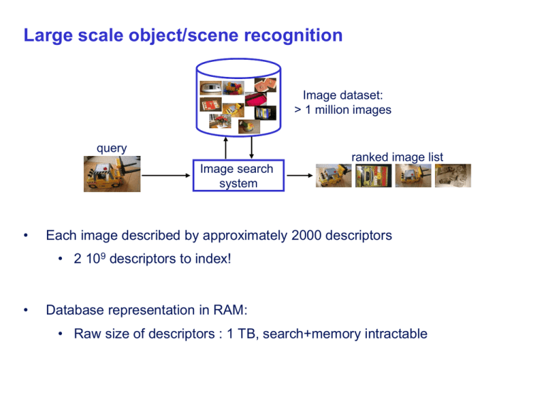
Large scale object/scene recognition
Image dataset:
> 1 million images
query
ranked image list
Image search
system
•
Each image described by approximately 2000 descriptors
• 2 109 descriptors to index!
•
Database representation in RAM:
• Raw size of descriptors : 1 TB, search+memory intractable
State-of-the-art: Bag-of-words [Sivic & Zisserman’03]
Query
image
Set of SIFT
descriptors
centroids
(visual words)
[Nister & al 04, Chum & al 07]
sparse frequency vector
Bag-of-features
processing
+tf-idf weighting
Hessian-Affine
regions + SIFT descriptors
[Mikolajezyk & Schmid 04]
[Lowe 04]
Two issues:
Inverted
file
querying
- Matching approximation by visual words
- Still limited number of images
Re-ranked
list
Geometric
verification
[Lowe 04, Chum & al 2007]
ranked image
short-list
Bag-of-features as an ANN search algorithm
•
Matching function of descriptors : k-nearest neighbors
•
Bag-of-features matching function
where q(x) is a quantizer, i.e., assignment to visual word and
δa,b is the Kronecker operator (δa,b=1 iff a=b)
Approximate nearest neighbor search evaluation
•
ANN algorithms usually returns a short-list of nearest neighbors
• this short-list is supposed to contain the NN with high probability
• exact search may be performed to re-order this short-list
•
Proposed quality evaluation of ANN search: trade-off between
• Accuracy: NN recall = probability that the NN is in this list
against
• Ambiguity removal = proportion of vectors in the short-list
• the lower this proportion, the more information we have about the vector
• the lower this proportion, the lower the complexity if we perform exact search on
the short-list
•
ANN search algorithms usually have some parameters to handle this trade-off
ANN evaluation of bag-of-features
0.7
ANN algorithms returns a
list of potential
neighbors
k=100
0.6
200
0.5
Accuracy: NN recall
= probability that the
NN is in this list
500
NN recall
1000
0.4
2000
Ambiguity removal:
= proportion of vectors
in the short-list
5000
0.3
10000
20000
30000
50000
0.2
In BOF, this trade-off is
managed by the
number of clusters k
0.1
0
1e-07
BOW
1e-06
1e-05
0.0001
0.001
rate of points retrieved
0.01
0.1
Problem with bag-of-features
•
•
The intrinsic matching scheme performed by BOF is weak
•
for a “small” visual dictionary: too many false matches
•
for a “large” visual dictionary: many true matches are missed
No good trade-off between “small” and “large” !
•
either the Voronoi cells are too big
•
or these cells can’t absorb the descriptor noise
 intrinsic approximate nearest neighbor search of BOF is not sufficient
20K visual word: false matchs
200K visual word: good matches missed
Hamming Embedding
•
Representation of a descriptor x
• Vector-quantized to q(x) as in standard BOF
+ short binary vector b(x) for an additional localization in the Voronoi cell
•
Two descriptors x and y match iif
where h(a,b) is the Hamming distance
•
Nearest neighbors for Hammg distance  the ones for Euclidean distance
•
Efficiency
• Hamming distance = very few operations
• Fewer random memory accesses: 3 faster that BOF with same dictionary size!
Hamming Embedding
•
Off-line (given a quantizer)
• draw an orthogonal projection matrix P of size db × d
 this defines db random projection directions
• for each Voronoi cell and projection direction, compute the median value
from a learning set
•
On-line: compute the binary signature b(x) of a given descriptor
• project x onto the projection directions as z(x) = (z1,…zdb)
• bi(x) = 1 if zi(x) is above the learned median value, otherwise 0
[H. Jegou et al., Improving bag of features for large scale image search, ICJV’10]
Hamming and Euclidean neighborhood
rate of 5-NN retrieved (recall)
1
•
0.8
trade-off between
memory usage and
accuracy
 more bits yield higher
accuracy
0.6
We used 64 bits (8 bytes)
0.4
0.2
0
8 bits
16 bits
32 bits
64 bits
128 bits
0
0.2
0.4
0.6
0.8
rate of cell points retrieved
1
ANN evaluation of Hamming Embedding
0.7
28 32
24
0.6
22
200
compared to BOW: at
least 10 times less points
in the short-list for the
same level of accuracy
20
0.5
500
1000
18
NN recall
k=100
0.4
2000
ht=16
0.3
5000
Hamming Embedding
provides a much better
trade-off between recall
and ambiguity removal
10000
20000
30000
50000
0.2
0.1
0
1e-08
HE+BOW
BOW
1e-07
1e-06
1e-05 0.0001 0.001
rate of points retrieved
0.01
0.1
Matching points - 20k word vocabulary
201 matches
Many matches with the non-corresponding image!
240 matches
Matching points - 200k word vocabulary
69 matches
Still many matches with the non-corresponding one
35 matches
Matching points - 20k word vocabulary + HE
83 matches
10x more matches with the corresponding image!
8 matches
Weak geometry consistency
Re-ranking based on full geometric verification [Lowe 04, Chum & al 2007]
•
works very well
•
but performed on a short-list only (typically, 100 images)
 for very large datasets, the number of distracting images is so high that
relevant images are not even short-listed!
1
short-list size:
rate of relevant images short-listed
•
0.9
20 images
100 images
0.8
1000 images
0.7
0.6
0.5
0.4
0.3
0.2
0.1
0
1000
10000
dataset size
100000
1000000
Weak geometry consistency
•
Weak geometric information used for all images (not only the short-list)
•
Each invariant interest region detection has a scale and rotation angle
associated, here characteristic scale and dominant gradient orientation
Scale change 2
Rotation angle ca. 20 degrees
•
Each matching pair results in a scale and angle difference
•
For the global image scale and rotation changes are roughly consistent
WGC: orientation consistency
Max = rotation angle between images
WGC: scale consistency
Weak geometry consistency
•
Integrate the geometric verification into the BOF representation
• votes for an image projected onto two quantized subspaces, that is vote
for an image at a given angle & scale
• these subspace are show to be independent
• a score sj for all quantized angle and scale differences for each image
• final score: filtering for each parameter (angle and scale) and min selection
•
Only matches that do agree with the main difference of orientation and scale
will be taken into account in the final score
•
Re-ranking using full geometric transformation still adds information in a final
stage
Experimental results
•
Evaluation for the INRIA holidays dataset, 1491 images
• 500 query images + 991 annotated true positives
• Most images are holiday photos of friends and family
•
1 million & 10 million distractor images from Flickr
•
Vocabulary construction on a different Flickr set
•
Almost real-time search speed
•
Evaluation metric: mean average precision (in [0,1], bigger = better)
• Average over precision/recall curve
Holiday dataset – example queries
Dataset : Venice Channel
Query
Base 1
Base 3
Base 2
Base 4
Dataset : San Marco square
Query
Base 1
Base 4
Base 5
Base 8
Base 9
Base 2
Base 6
Base 3
Base 7
Example distractors - Flickr
Experimental evaluation
•
Evaluation on our holidays dataset, 500 query images, 1 million distracter
images
•
Metric: mean average precision (in [0,1], bigger = better)
1
baseline
0.9
0.8
HE
+re-ranking
0.7
mAP
0.6
0.5
0.4
0.3
0.2
0.1
0
1000
10000
100000
database size
1000000
Query
BOF 2
Ours 1
BOF 5890
Ours 4
BOF 43064
Ours 5
Results – Venice Channel
Base 1
Flickr
Query
Flickr
Base 4
Comparison with the state of the art: Oxford dataset [Philbin et al. CVPR’07]
Evaluation measure:
Mean average precision (mAP)
Comparison with the state of the art: Kentucky dataset [Nister et al. CVPR’06]
4 images per object
Evaluation measure: among the 4 best retrieval results how
many are correct (ranges from 1 to 4)
Comparison with the state of the art
[14] Philbin et al., CVPR’08;
[6] Nister et al., CVPR’06;
[10] Harzallah et al., CVPR’07
Demo at http://bigimbaz.inrialpes.fr
Extension to videos: video copy detection

Recognized “attacked” videos (distortion, blur, editing, mix up,...)
•a few seconds
•1000 of hours


Video = image sequence: use image indexing
►
index frames / keyframes of video, query frames of video query
►
verify temporal consistency
Several tradeoffs in search quality vs. database size
Temporal consistency

Store a subset of the frames of the video to be indexed in a database

Each frame of the query video is compared to the frames in the dataset of
frames
→ Output: a set of matching frames and associated scores (tq, b, tb , s) where
tq
b
tb
s
temporal position in the query video
number of the video in the dataset
temporal position in the database video
matching score for the two frames
Temporal consistency

Estimate a function between tq and tb

Possible models:
►
simple (temporal shift): tq = tb + t
►
global speed changes (acceleration, slow-motion): tq =a* tb + t
►
complex with varying shifts: tq = tb + shift [tq]
Temporal consistency

Estimate a function between tq and tb

Possible models:
►
simple (temporal shift): tq = tb + t

►
global speed changes (acceleration, slow-motion): tq =a* tb + t
►
complex with varying shifts: tq = tb + shift [tq]
Possible method for estimation:
►
Hough transform
TrecVid’08 copyright detection competition
precision
Precision-recall: combined transformation (10)
0.6
0.4
0.2
INRIA-LEAR.Strict
INRIA-LEAR.Soft
INRIA-LEAR.KeysAds
Others
Others
0
0
0.2
0.4
0.6
recall
Sample result
Sample result
Towards larger databases?

BOF can handle up to ~10 M d’images
►
with a limited number of descriptors per image
►
40 GB of RAM
►
search = 2 s

Web-scale = billions of images
►
With 100 M per machine
→ search = 20 s, RAM = 400 GB
→ not tractable!
State-of-the-art: Bag-of-words [Sivic & Zisserman’03]
Query
image
Set of SIFT
descriptors
centroids
(visual words)
[Nister & al 04, Chum & al 07]
sparse frequency vector
Bag-of-features
processing
+tf-idf weighting
Hessian-Affine
regions + SIFT descriptors
[Mikolajezyk & Schmid 04]
[Lowe 04]

“visual words”:
►
1 “word” (index) per local descriptor
►
only images ids in inverted file
Re-ranked
list
Inverted
file
Geometric
verification
[Lowe 04, Chum & al 2007]
querying
ranked image
short-list
Recent approaches for very large scale indexing
Query
image
Set of SIFT
descriptors
centroids
(visual words)
sparse frequency vector
Bag-of-features
processing
+tf-idf weighting
Hessian-Affine
regions + SIFT descriptors
Vector
compression
Vector
search
Re-ranked
list
Geometric
verification
ranked image
short-list
Related work on very large scale image search





Min-hash and geometrical min-hash [Chum et al. 07-09]
Compressing the BoF representation (miniBof) [ Jegou et al. 09]
 require hundreds of bytes are required to obtain a “reasonable quality”
GIST descriptors with Spectral Hashing [Weiss et al.’08]
 very limited invariance to scale/rotation/crop
Global scene context – GIST descriptor

The “gist” of a scene: Oliva & Torralba (2001)

5 frequency bands and 6 orientations for each image location
PCA or tiling of the image (windowing) to reduce the dimension

GIST descriptor + spectral hashing

The position of the descriptor in the image is encoded in the representation
•Gist
•Torralba et al. (2003)

Spectral hashing produces binary codes similar to spectral clusters
Related work on very large scale image search



Min-hash and geometrical min-hash [Chum et al. 07-09]
Compressing the BoF representation (miniBof) [ Jegou et al. 09]
 require hundreds of bytes are required to obtain a “reasonable quality”

GIST descriptors with Spectral Hashing [Weiss et al.’08]
 very limited invariance to scale/rotation/crop

Aggregating local descriptors into a compact image representation [Jegou et al. ‘10]

Efficient object category recognition using classemes [Torresani et al.’10]

Aggregating local descriptors into a compact image representation

Aim: improving the tradeoff between
►
search speed
►
memory usage
►
search quality

Approach: joint optimization of three stages
►
local descriptor aggregation
►
dimension reduction
►
indexing algorithm
Image representation
VLAD
PCA +
PQ codes
(Non) – exhaustive
search
Aggregation of local descriptors

Problem: represent an image by a single fixed-size vector:
set of n local descriptors → 1 vector
Most popular idea: BoF representation [Sivic & Zisserman 03]
►
sparse vector
►
highly dimensional
→ high dimensionality reduction/compression introduces loss


Alternative : vector of locally aggregated descriptors (VLAD)
►
non sparse vector
►
excellent results with a small vector dimensionality
VLAD : vector of locally aggregated descriptors

Learning: a vector quantifier (k-means)
►
output: k centroids (visual words): c1,…,ci,…ck
►
centroid ci has dimension d

For a given image
►
assign each descriptor to closest center ci
►
accumulate (sum) descriptors per cell
vi := vi + (x - ci)

x
VLAD (dimension D = k x d)
ci

The vector is L2-normalized
VLADs for corresponding images
v1
v2
v3 ...
SIFT-like representation per centroid (+ components: blue, - components: red)

good coincidence of energy & orientations
VLAD performance and dimensionality reduction


We compare VLAD descriptors with BoF: INRIA Holidays Dataset (mAP,%)
Dimension is reduced to from D to D’ dimensions with PCA (principal
component analyses)
Aggregator
k
D
D’=D
D’=128
D’=64
(no reduction)

BoF
1,000
1,000
41.4
44.4
43.4
BoF
20,000
20,000
44.6
45.2
44.5
BoF
200,000
200,000
54.9
43.2
41.6
VLAD
16
2,048
49.6
49.5
49.4
VLAD
64
8,192
52.6
51.0
47.7
VLAD
256
32,768
57.5
50.8
47.6
Observations:
►
VLAD better than BoF for a given descriptor size
►
Choose a small D if output dimension D’ is small
Compact image representation

Approach: joint optimization of three stages
►
local descriptor aggregation
►
dimension reduction
►
indexing algorithm
Image representation
VLAD
►
PCA +
PQ codes
(Non) – exhaustive
search
Dimensionality reduction with
►
Principal component analysis (PCA)
►
Compact encoding: product quantizer
►
 very compact descriptor, fast nearest neighbor search, little storage
requirements
Product quantization

Vector split into m subvectors:

Subvectors are quantized separately by quantizers
where each is learned by k-means with a limited number of centroids

Example: y = 128-dim vector split in 8 subvectors of dimension 16
►
each subvector is quantized with 256 centroids -> 8 bit
►
very large codebook 256^8 ~ 1.8x10^19
16 components
y1
y2
y3
y4
y5
y6
y7
y8
256
q
centroids 1
q2
q3
q4
q5
q6
q7
q8
q2(y2)
q3(y3)
q4(y4)
q5(y5)
q6(y6)
q7(y7)
q8(y8)
q1(y1)
8 bits
⇒ 8 subvectors x 8 bits = 64-bit quantization index
Product quantizer: distance computation

Asymmetric distance computation (ADC)

Sum of square distances with quantization centroids
Product quantizer: asymmetric distance computation (ADC)

Compute the square distance approximation in the compressed domain

To compute distance between query
and many codes
►
compute
for each subvector
and all possible centroids
→ stored in look-up tables
►
for each database code: sum the elementary square distances

Each 8x8=64-bits code requires only m=8 additions per distance!
Optimizing the dimension reduction and quantization together


VLAD vectors suffer two approximations
►
mean square error from PCA projection:
►
mean square error from quantization:
ep(D’)
eq(D’)
Given k and bytes/image, choose D’ minimizing their sum
Ex, k=16, 16B:
D’
ep(D’)
eq(D’)
ep(D’)+eq(D’)
32
0.0632
0.0164
0.0796
48
0.0508
0.0248
0.0757
64
0.0434
0.0321
0.0755
80
0.0386
0.0458
0.0844
Joint optimization of VLAD and dimension reduction-indexing

For VLAD
►
The larger k, the better the raw search performance
►
But large k produce large vectors, that are harder to index

Optimization of the vocabulary size
►
Fixed output size (in bytes)
►
D’ computed from k via the joint optimization of reduction/indexing
►
Only k has to be set
 end-to-end parameter optimization
Results on the Holidays dataset with various quantization parameters
Results on standard datasets

Datasets
►
University of Kentucky benchmark
►
INRIA Holidays dataset
Method
score: nb relevant images, max: 4
score: mAP (%)
bytes
UKB
Holidays
BoF, k=20,000
10K
2.92
44.6
BoF, k=200,000
12K
3.06
54.9
miniBOF
20
2.07
25.5
miniBOF
160
2.72
40.3
VLAD k=16, ADC 16 x 8
16
2.88
46.0
VLAD k=64, ADC 32 x10
40
3.10
49.5
D’ =64 for k=16 and D’ =96 for k=64
ADC (subvectors) x (bits to encode each subvector)
miniBOF: “Packing Bag-of-Features”, ICCV’09
Comparison BOF / VLAD + ADC

Datasets
►
INRIA Holidays dataset , score: mAP (%)
Method
Holidays
BOF, k=2048, D’= 64, ADC 16x8
42.5
VLAD k=16,D=2048, D’ = 64, ADC 16 x 8
46.0
BOF, k=8192, D’= 128, AD16x8
41.9
VLAD k=64, D= 8192, D’=128, ADC 16X8
45.8
►
►
VLAD improves results over BOF
Product quantizer gives excellent results for BOF!
Compact image representation


Approach: joint optimization of three stages
Non-exhaustive search
►
local descriptor aggregation
►
dimension reduction
►
indexing algorithm
Image representation
VLAD

PCA +
PQ codes
(Non) – exhaustive
search
Non-exhaustive search
►
Combination with an inverted file to avoid exhaustive search
Large scale experiments (10 million images)

Exhaustive search of VLADs, D’=64
►
4.77s

With the product quantizer
►
Exhaustive search with ADC:
0.29s
►
Non-exhaustive search with IVFADC: 0.014s
IVFADC -- Combination with an inverted file
Large scale experiments (10 million images)
0.8
0.7
0.6
recall@100
0.5
Timings
0.4
4.768s
0.3
0.2
0.1
ADC:
0.286s
IVFADC: 0.014s
BOF D=200k
VLAD k=64
VLAD k=64, D'=96
VLAD k=64, ADC 16 bytes
VLAD+Spectral Hashing, 16 bytes
0
1000
10k
100k
1M
Database size: Holidays+images from Flickr
SH ≈ 0.267s
10M
Searching with quantization: comparison with spectral Hashing

*** Put Only ADC ***
VLAD + PQ codes

Excellent search accuracy and speed in 10 million of images

Each image is represented by very few bytes (20 – 40 bytes)

Tested on up to 220 million video frame
►
extrapolation for 1 billion images: 20GB RAM, query < 1s on 8 cores

On-line available:
►
Matlab source code of ADC

Alternative: using Fisher vectors instead of VLAD descriptors [Perronnin’10]