Mixed Precision Iterative Refinement Solver Procedure
Using High Performance Linpack (HPL)
H. Che2, E. D’Azevedo1, M. Sekachev3, K. Wong3
1Oak Ridge National Laboratory, 2Chinese University of Hong Kong, 3National Institute for Computational Sciences
Motivation
• Single Instruction Multiple Data (SIMD) capability in most processors
can achieve higher performance in 32-bit over 64-bit operations.
=> Iterative refinement procedure
Goals
• Deliver a user library by extending HPL to perform single, double,
complex, double complex, and mixed precisions calculations.
• Deliver an interface compatible to ScaLAPACK calling convention,
which allows simple code modifications to achieve top performance
using this modified HPL (libmhpl.a) library.
• Use mixed precision solver by performing costly LU factorization in 32bit but achieve 64-bit accuracy by iterative refinement method.
•
•
/*
* Find norm_1( A ).
*/
if( nq > 0 )
{
float*
float
work = (double*)malloc( nq * sizeof( double ) );
if( work == NULL )
HPL_pslange
{ HPL_pabort( __LINE__, "HPL_pdlange", "Memory allocation
failed" ); }
•
High Performance Linpack (HPL)
• HPL is written in portable C to evaluate parallel performance of Top500
computers by solving a (random) dense linear system in double
precision (64-bit) arithmetic on distributed-memory computers.
• HPL uses a right-looking variant of the LU factorization of random
matrix with row partial pivoting. 2-D block-cyclic distribution is
employed.
• It has tunable parameters to implement multiple look-ahead depths,
recursive panel factorization with pivot search and column broadcast
combined, various virtual panel broadcast topologies, bandwidth
reducing swap broadcast algorithm, and a ring broadcast algorithm in
the backward substitution
Data-type Change:
• Variable Data-type: double A → double complex A
• MPI communication Data-type:
MPI_Send(A,…,MPI_DOUBLE,…) →
MPI_Send(A,…,MPI_DOUBLE_COMPLEX,…)
• Function return type:
double HPL_rand →
double complex HPL_zrand
For example, HPL_pdlange.c becomes HPL_pslange.c
with the following change in content:
for( jj = 0; jj < nq; jj++ )
{
(float)HPL_rzero
s = HPL_rzero;
for( ii = 0; ii < mp; ii++ ) { s += Mabs( *A ); A++; }
work[jj] = s; A += LDA - mp;
}
Unchanged:
• Timing variables: /hpl/testing /ptimer, /timer
• Norm Variables: Anorm1 in HPL_pztest.c
• Residue Variables: resid0 in HPL_pztest.c
• Function return Data-type: double HPL_pzlange
ScaLAPACK Based Application Code Modifications
• Performing simple modifications of ScaLAPACK source codes one can
embed calling more efficient HPL functions, simply linked with
libmhpl.a provided here.
• For example the test program provided by ScaLAPACK
(pdludriver.f) should be modified as follow as follows
(pdhpl_driver.f):
1. Two extra integers are declared:
integer
Numerical Experiments
•
•
Precision
SINGLE
REAL
Processor
Grid
(P x Q)
Size of
matrix
(N)
DOUBLE
COMPLEX
TEMPLATE DESIGN © 2008
www.PosterPresentations.com
•
•
40.81
29.45
11.63
15.65
80,000
64.07
44.28
16.22
21.61
160,000
226.45
132.0
44.44
55.34
320,000
519.16
285.82
99.09
118.23
115.42
70.09
44.40
50.72
73.23
48.50
20.99
26.79
128 x 128
64.07
44.28
16.22
21.61
SCALAPACK
(p?ludriver.f)
32 x 32
638.28
343.80
261.53
275.89
HPL
309.83
178.09
92.31
104.06
226.45
132.0
44.44
55.34
64 x 64
80,000
160,000
128 x 128
19,876.20
18.84
6.59
320,000
108,016.90
39,493.40
35.83
13.10
640,000
174,400.00
-
57.85
-
1,200,000
211,600.00
-
70.19
-
5,000
33.47
27.67
45.48
37.60
14,000
46.72
42.37
63.48
57.57
80,000
14,034.10
5,095.30
4.66
1.69
160,000
36,361.10
11,683.00
12.06
3.88
320,000
61,095.40
21,471.60
20.27
7.12
640,000
92,980.00
-
40.84
-
1,200,000
106,600.00
-
35.36
-
5,000
18.79
15.28
51.06
41.52
40,000
38.30
25.25
9.92
12.98
14,000
24.40
20.41
66.30
55.46
60,000
73.55
46.72
17.39
20.98
80,000
48,224.60
17,631.80
16.00
5.88
80,000
122.18
75.82
25.32
31.46
160,000
103,168.20
38,515.40
34.22
12.78
160,000
480.54
260.62
102.43
119.03
320,000
150,771.10
69,657.70
50.01
23.11
320,000
1171.44
630.62
272.26
307.06
640,000
211,100.00
-
70.02
-
32 x 32
333.22
194.45
134.88
145.18
5,000
44.59
34.93
60.58
47.46
64 x 64
163.18
100.17
43.58
60.46
14,000
54.40
47.11
73.91
64.01
128 x 128
122.18
75.82
25.32
31.46
80,000
32,262.60
10,702.20
10.70
3.55
32 x 32
2046.90
1103.87
898.28
927.84
160,000
56,937.20
21,813.70
18.87
7.23
64 x 64
799.02
443.89
275.53
300.67
320,000
79,678.70
37,673.60
26.43
12.50
128 x 128
480.54
260.62
102.43
119.03
5,000
23.40
18.91
63.59
51.39
14,000
27.37
24.33
74.36
66.11
128 x 128
2x2
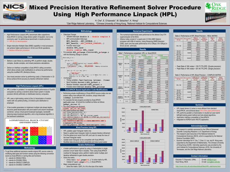
• Peak Rate of 16K nodes = 150.73 TFLOPS (Double precision)
• Peak Rate of 16K nodes = 301.46 TFLOPS (Single precision)
Table 3: Performance of HPL Mixed Precision – COMPLEX MATRIX
Processor Grid
(P x Q)
128 x 128
Size of matrix
(N)
COMPLEX*16
ScaLAPACK
LU, sec
80,000
160,000
COMPLEX*8
ScaLAPACK
LU, sec
COMPLEX*8
HPL
LU, sec
Mixed
Precision
Solve, sec
Summary
SCALAPACK
HPL
• HPL based dense LU solver is more efficient than standard
ScaLAPACK, and achieved about 75% of the peak performance.
• HPL performs parallel LU factorization in double but uses hybrid
left/right-looking panel method and look-ahead algorithms.
• Application interface compatible to ScaLAPACK.
• Integrated to AORSA fusion INCITE application.
120,000
SINGLE REAL
DOUBLE REAL
100,000
80,000
60,000
40,000
Acknowledgements
20,000
•
0
80,000
160,000
320,000
80,000
160,000
320,000
Matrix Dimension (N)
SCALAPACK
•
HPL
160,000
DOUBLE COMPLEX
SINGLE COMPLEX
140,000
120,000
100,000
GFLOPS
• To get three additional precisions rewrite original HPL source codes by
modifying data types and function names using the following convention
(same as ScaLAPACK) in naming files and functions:
‘s’ – stands for SINGLE REAL
‘d’ – stands for DOUBLE REAL
‘c’ – stands for SINGLE COMPLEX
‘z’ – stands for DOUBLE COMPLEX
60,000
56,810.50
128 x 128
z
HPL updates upper triangular matrix only
Need to update lower triangular matrix to prepare iterative refinement
Find the global pivot vector from HPL and use it to swap the rows of
the lower triangular matrix
Update lower triangular (to be compatible with ScaLAPACK)
Modified data structure code to assemble and return pivot vector
A better performance is gained by using LU factorization in single
precision (much faster than in double). Then using ScaLAPACK
routines for triangular solve, perform matrix-vector multiply and
iterative refinement to gain double precision.
Solve the matrix
− Using ‘call hpl_psgesv(…)’ to solve matrix by HPL
− Instead of ‘call psgetrf(…)’ (ScaLAPACK)
Major computational cost
− Solve the matrix: O(N3), N x N is the size of the matrix
10.17
160,000
2x2
Iterative Refinement
•
7.48
2.52
c
Mixed Precision Using HPL
Methodology
17.20
6.16
2x2
SINGLE
COMPLEX
SCALAPACK
(p?ludriver.f)
Mixed
Precision
Solve, sec
7,586.00
128 x 128
d
HPL
% of peak
REAL*4
HPL
LU, sec
18,565.90
2x2
DOUBLE
REAL
GFLOPS
REAL*4
ScaLAPACK
LU, sec
22.91
64 x 64
call hpl_pdgesv(n, mem(IPA), descA,mem(ippiv), info)
•
•
REAL*8
ScaLAPACK
LU, sec
80,000
128 x 128
s
is replaced by HPL function
•
•
•
Size of matrix
(N)
40,000
128 x 128
Table 1: Performance comparison: HPL vs. ScaLAPACK
blacs_barrier(ictxt,'A')
hpl_dblacsinit( ictxt )
hpl_dmatinit( n, NB, hpl_lld,hpl_ineed)
descinit(descA,n,n+1,NB,NB,0,0,ICTXT,hpl_lld,ierr(1))
CALL PDGETRF(M,N,MEM(IPA),1,1,DESCA,MEM(IPPIV),INFO )
Processor Grid
(P x Q)
32 x 32
hpl_lld, hpl_ineed
3. Original ScaLAPACK function
Table 2: Performance of HPL Mixed Precision – REAL MATRIX
Results
2. HPL extra functions are called:
call
call
call
call
Results
The numerical experiments were performed on the athena Cray XT4
supercomputer at the NICS.
Athena nodes consist of a quad-core 2.3 GHz AMD Opteron
processor with 4GB of memory. Using Streaming SIMD Extension
(SSE), each core has peak performance of 9.2 Gflops (18.4 Gflops) in
64-bit (32-bit) arithmetic.
GFLOPS
• High Performance Linpack (HPL) benchmark often outperforms
ScaLAPACK in solving a large dense system of equation, but is only
commonly used for performance benchmark in double precision.
=> HPL for LU decomposition
Methodology
80,000
•
This research is partially sponsored by the Office of Advanced
Scientific Computing Research; U.S. Department of Energy.
This research used resources of the National Institute for
Computational Sciences (NICS), which is supported by the National
Science Foundation (NSF).
Summer internships for H. Che, T. Chan, D. Lee, and R. Wong were
supported by the Department of Mathematics, The Chinese University
of Hong Kong (CUHK). Internship opportunity was provided by the
Joint Institute for Computational Sciences (JICS), the University of
Tennessee, and the Oak Ridge National Laboratory.
60,000
Contact information
40,000
20,000
0
80,000
160,000
320,000
80,000
Matrix Dimension (N)
160,000
320,000
Eduardo F. D’Azevedo, ORNL
Kwai Wong, NICS
E-mail: e6d@ornl.gov
E-mail: wong@jics.utk.edu
http://www.nics.utk.edu/sites/default/files/HPL-site/home.html