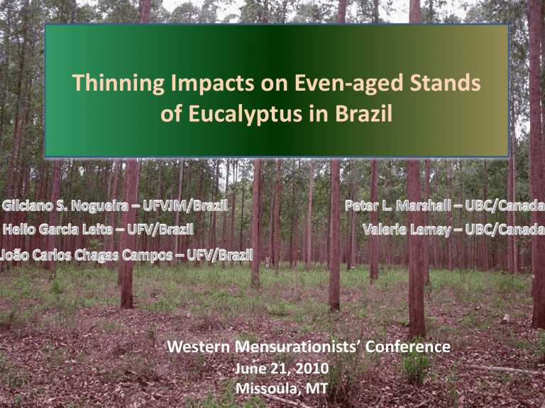
Thinning Impacts on Even-aged Stands
of Eucalyptus in Brazil
Western Mensurationists’ Conference
June 21, 2010
Missoula, MT
Introduction
Plantation forest in Brazil: 6.6 million hectares, representing 0.8 % of the land area
From 2004 to 2008 the area in eucalyptus plantation increased by 33.1%, or 1.1 million ha
solid wood products is minimal
Introduction
Advances in wood technology and design have allowed various uses of eucalyptus
wood as a solid product
Introduction
The demand for wood from large trees has been supported by illegal harvesting in
native forests
Consequently, there are also few studies on the impact of thinning in stands of
eucalyptus in Brazil
Introduction
Thinning in eucalyptus forests can help increase Brazilian participation in the
global market for solid wood products and may reduce pressure on Brazilian native
forests
Studies of thinning in eucalyptus are strategic for Brazil, both economically and
environmentally
Introduction
An experiment was established to obtain a database reliable for analyzing the
difference among thinning treatments and for developing growth and yield models for
thinned eucalyptus stands
Requirements:
- Selection of the sample units was deliberate (selective sampling), so that
representation of the medium and extreme site conditions is guaranteed
- The sample units were sufficiently large to faithfully represent the silvicultural
practices applied to the remainder of the stand
Objective
To analyze the effect of thinning on growth of stand
variables in eucalyptus forests
Overview of the experiment
- Species: Eucalyptus grandis x Eucalyptus urophylla hybrid
- Location: Northeast region of Bahia State, Brazil
Overview of the experiment
- Planting date: June/July 1993
- Date of installation of the permanent plots: September 1995
- Company: Bahia Specialty Cellulose (BSC) (http://www.bahiaspeccell.com)
- Initial spacing between trees: 3.0 X 3.0 m
- Thinnings accomplished: two selective thinnings, in 1998 and 2004
- Final harvest: at the end of 2007
Experimental Design
- based on level-of-growing-stock installation standards
- Located in 3 installations, comprising medium and good quality site conditions
Experimental Design
- Replicated randomized complete block with repeated measures
- 6 blocks (two in each installation), each one involving two repetitions;
- 4 treatments, corresponding to different basal area percentages removed in each thinning :
Treatment 1: 20% without pruning;
Treatment 2: 35% without pruning;
Treatment 3: 50% without pruning;
Treatment 4: 35% with pruning up to 6.0 meters;
- Each block contained 8 permanent rectangular plots, with an area of 2,600 m2, totaling 48
plots (6 blocks x 2 repetitions x 4 treatments)
Experimental Design
- Layout
C
Block 1
A
Block 1
B
Block 1
Block 2
99,28
99,28
3
2
2
1
3
2
1
4
204,0 m
204,0 m
Block 2
1
4
4
3
4
3
2
1
I
II
III
IV
119.0 m
3
2
2
1
1
4
176.8 m
4
3
III
IV
Block 2
Experimental Design
- Replicated randomized complete block with repeated measures
- 6 blocks (two in each installation), each one involving two repetitions;
- 4 treatments, corresponding to different basal area percentages removed in each thinning :
Treatment 1: 20% without pruning;
Treatment 2: 35% without pruning;
Treatment 3: 50% without pruning;
Treatment 4: 35% with pruning up to 6.0 meters;
- Each block contained 8 permanent rectangular plots, with an area of 2,600 m2, totaling 48
plots (6 blocks x 2 repetitions x 4 treatments)
- Plots were buffered by a few rows of trees on each side
Marked boundaries of a plot
Measurements
- Data
1
2
3
4
Year of
measurement
1995
1996
1997
1998
5
6
7
8
9
10
11
12
13
1999
2000
2001
2002
2003
2004
2005
2006
2007
Measurement
Age
(month)
27
40
50
Age
(year)
61
75
87
100
111
124
136
147
157
164
5.1
6.3
7.3
8.3
9.3
10.3
11.3
12.3
13.1
13.7
2.3
3.3
4.2
Note
before 1st thinning
before 1st thinning
before 1st thinning; 1st stem analysis (6 trees per dbh class)
after 1st thinning
after 1st thinning
after 1st thinning
after 1st thinning
after 1st thinning
after 1st thinning
after 1st thinning
after 2nd thinning
after 2nd thinning
after 2nd thinning; 2nd stem analysis (6 trees per dbh class)
Measurements
After 1st thinning (61 months)
After 1st thinning (101 months)
After 1st thinning (87 months)
After 2nd thinning (165 months)
Volume equation
outside bark:
LnVt   -10.28859  1.751165Lndbh  1.23523LnHt 
R 2  0.998
inside bark:
LnVt   -10.39158  1.74249Lndbh  1.22368LnHt 
R 2  0.998
Volume equation
outside bark
Distribution of Raw residuals
Predicted vs. Observed Values
Expected Normal
Predicted vs. Residual Scores
Dependent variable: LnVtob
200
Dependent variable: LnVtob
180
0.0
0.20
160
-0.5
0.15
140
-1.0
0.10
120
-1.5
0.05
100
-2.0
0.00
80
-2.5
-0.05
60
40
20
0
-0.30
-0.25
-0.20
-0.15
-0.10
-0.05
0.00
0.05
0.10
0.15
0.20
-3.0
-0.10
-3.5
-0.15
-4.0
-0.20
-4.5
-4.5
0.25
Residuals
0.25
Observed Values
No of obs
0.5
-4.0
-3.5
-3.0
-2.5
-2.0
-1.5
-1.0
-0.5
Predicted Values
0.0
-0.25
0.5
-5
-4
-3
95% confidence
-2
-1
0
Predicted Values
95% confidence
inside bark
Distribution of Raw residuals
Predicted vs. Observed Values
Expected Normal
Predicted vs. Residual Scores
Dependent variable: LnVtib
Dependent variable: LnVtib
0.25
180
-0.5
0.20
160
-1.0
0.15
140
-1.5
0.10
120
-2.0
0.05
100
-2.5
0.00
80
-3.0
-0.05
60
40
20
0
-0.30
-0.25
-0.20
-0.15
-0.10
-0.05
0.00
0.05
0.10
0.15
0.20
Residuals
0.0
Observed Values
No of obs
200
-3.5
-0.10
-4.0
-0.15
-4.5
-0.20
-5.0
-5.0
-4.5
-4.0
-3.5
-3.0
-2.5
-2.0
Predicted Values
-1.5
-1.0
-0.5
0.0
95% confidence
-0.25
-5.0
-4.5
-4.0
-3.5
-3.0
-2.5
-2.0
Predicted Values
-1.5
-1.0
-0.5
0.0
95% confidence
Height equation
Installation A
LnHt   -29.32738  0.42280 Ln Age - 0.00231Age  12.92836 LnSI   -0.49355SI 
0.64171Lndbh   -0.01683dbh
R 2  0.97
Installation B
LnHt   -38.23811 0.45930 Ln Age - 0.00238 Age  17.21817 LnSI   0.68722SI 
0.54414 Lndbh  - 0.01233dbh
R 2  0.97
Installation C
LnHt   -32.40495  0.85823Ln Age - 0.00774 Age  12.67110 LnSI   0.41164 SI 
0.81710 Lndbh  - 0.03013dbh
R 2  0.98
Height equation
A
Predicted vs. Observed Values
Distribution of Raw residuals
Expected Normal
Dependent variable: LnHt
Predicted vs. Residual Scores
0.20
700
3.4
0.15
600
3.2
0.10
500
3.0
0.05
400
2.8
0.00
300
2.6
-0.05
200
100
0
-0.20
-0.16
-0.12
-0.08
-0.04
0.00
0.04
0.08
0.12
0.16
0.20
Residuals
3.6
Observed Values
No of obs
800
-0.10
2.4
-0.15
2.2
2.0
2.0
2.2
2.4
2.6
2.8
3.0
3.2
3.4
Predicted Values
-0.20
2.0
3.6
2.2
2.4
2.6
2.8
3.0
3.2
Predicted Values
95% confidence
3.4
3.6
95% confidence
B
Predicted vs. Residual Scores
Predicted vs. Observed Values
Distribution of Raw residuals
Expected Normal
Dependent variable: LnHt
Dependent variable: LnHt
0.20
700
3.4
0.15
600
3.2
0.10
500
3.0
0.05
400
2.8
0.00
300
2.6
200
100
0
-0.20
-0.16
-0.12
-0.08
-0.04
0.00
0.04
0.08
0.12
0.16
0.20
Residuals
3.6
Observed Values
No of obs
800
2.4
-0.10
-0.15
2.2
2.0
2.0
-0.05
2.2
2.4
2.6
2.8
Predicted Values
3.0
3.2
3.4
3.6
95% confidence
-0.20
2.0
2.2
2.4
2.6
2.8
Predicted Values
3.0
3.2
3.4
3
95% confiden
Height equation
C
Distribution of Raw residuals
Predicted vs. Residual Scores
Predicted vs. Observed Values
Expected Normal
Dependent variable: LnHt
Dependent variable: LnHt
400
3.6
0.20
350
3.4
0.15
3.2
300
0.10
3.0
0.05
250
2.8
0.00
200
2.6
100
50
0
-0.20
-0.16
-0.12
-0.08
-0.04
0.00
0.04
0.08
0.12
0.16
0.20
Residuals
Observed Values
No of obs
150
2.4
2.2
-0.10
-0.15
2.0
1.8
1.8
-0.05
2.0
2.2
2.4
2.6
2.8
Predicted Values
3.0
3.2
3.4
3.6
95% confidence
-0.20
2.0
2.2
2.4
2.6
2.8
Predicted Values
3.0
3.2
3.4
3.6
95% confidence
Growth trend
Individual values
Mean per treatment
Growth trends
Individual values
Mean per treatment
Growth trends
Individual values
Mean per treatment
Growth trends
Individual values
Mean per treatment
Analysis
Variables:
- periodic monthly increment (absolute): total height, dominant height,
quadratic mean diameter and volume per tree
- periodic monthly increment (percentage): basal area per hectare and
volume per hectare
Periods:
A and B
1
2
3
(61 to 87) (87 to 137) (147 to 165)
C
1
2
(61 to 87) (61 to 87)
Analysis
Anova: Mixed linear model, with thinning as the whole plot factor and period as the
split-plot factor
Fixed effect: thinning
Random effect: block
block*thinning
Repetition(block*thinning)
period
period*thinning
Pairwise comparisons: Bonferroni test
Effect on periodic increment of average total height
There is thinning effect
A
B
A: only thinning 35% and thinning 35% + pruning were equal
B and C : Only thinning 20% was different from the other treatments
C
Effect on periodic increment of dominant height
No thinning effect
Effect on periodic increment of quadratic mean
diameter
There is thinning effect
A
B
A, B and C: only thinning 35% and thinning 35% + pruning were equal
C
Effect on periodic increment of basal area per
hectare
There is thinning effect
A
B
A, B and C: only thinning 35% and thinning 35% + pruning were equal
C
Effect on periodic increment of volume per hectare
There is thinning effect
A
B
A, B and C: only thinning 35% and thinning 35% + pruning were equal
C
Effect on periodic increment of volume per tree
There is thinning effect
A
B
A, B and C: only thinning 35% and thinning 35% + pruning were equal
C
Conclusion
No surprise!
Conclusion
Thinning affected the growth of total height, diameter, basal area per hectare, total
volume per tree and total volume per hectare, but did not affect the growth of
dominant height
Thinning prevented regular tree mortality
Prunning did not affect the growth trend of the variables analyzed
nogueirags@gmail.com