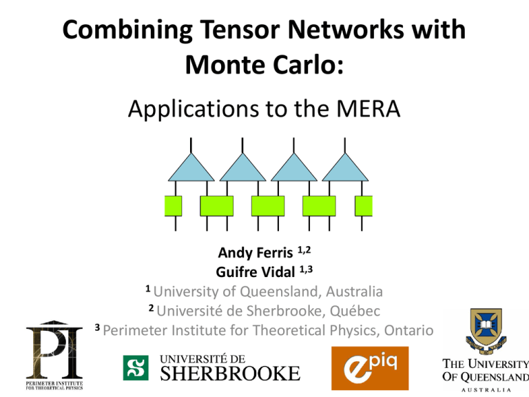
Combining Tensor Networks with
Monte Carlo:
Applications to the MERA
Andy Ferris 1,2
Guifre Vidal 1,3
1 University of Queensland, Australia
2 Université de Sherbrooke, Québec
3 Perimeter Institute for Theoretical Physics, Ontario
Motivation: Make tensor networks faster
χ
ys s s s s s s
1 2 3 4 5 6 7
Parameters: dL
vs.
Poly(χ,d,L)
Calculations should be efficient in memory and
computation (polynomial in χ, etc)
However total cost might still be HUGE (e.g. 2D)
Monte Carlo makes stuff faster
• Monte Carlo: Random sampling of a sum
– Tensor contraction is just a sum
• Variational MC: optimizing parameters
• Statistical noise!
1
Error µ
N
– Reduced by importance sampling over some
positive probability distribution P(s)
æ E(s) ö
E = å E(s) = å P(s). ç
÷
è P(s) ø
s
s
Monte Carlo with Tensor networks
Monte Carlo with Tensor networks
E = å E(s)
s
æ E(s) ö
E = å P(s). ç
÷
è P(s) ø
s
P(s) = Y s
2
Var[E(s) / P(s)]
< Var[E(s)]
Monte Carlo with Tensor networks
MPS: Sandvik and Vidal, Phys. Rev. Lett. 99, 220602 (2007).
CPS: Schuch, Wolf, Verstraete, and Cirac, Phys. Rev. Lett. 100, 040501 (2008).
Neuscamman, Umrigar, Garnet Chan, arXiv:1108.0900 (2011), etc…
PEPS: Wang, Pižorn, Verstraete, Phys. Rev. B 83, 134421 (2011). (no variational)
…
s
E = å E(s)
æ E(s) ö
E = å P(s). ç
÷
è P(s) ø
s
P(s) = Y s
2
Var[E(s) / P(s)]
< Var[E(s)]
Monte Carlo with Tensor networks
MPS: Sandvik and Vidal, Phys. Rev. Lett. 99, 220602 (2007).
CPS: Schuch, Wolf, Verstraete, and Cirac, Phys. Rev. Lett. 100, 040501 (2008).
Neuscamman, Umrigar, Garnet Chan, arXiv:1108.0900 (2011), etc…
PEPS: Wang, Pižorn, Verstraete, Phys. Rev. B 83, 134421 (2011). (no variational)
…
s
æ E(s) ö
Unitary TN: Ferris and Vidal, Phys. Rev. B 85, 165146 (2012).
1D MERA: Ferris and Vidal, Phys. Rev. B, 85, 165147
E (2012).
= P(s). ç
÷
E = å E(s)
å
s
P(s) = Y s
è P(s) ø
2
Var[E(s) / P(s)]
< Var[E(s)]
Perfect vs. Markov chain sampling
•
•
•
•
Perfect sampling: Generating s from P(s)
Often harder than calculating P(s) from s!
Use Markov chain update
e.g. Metropolis algorithm:
– Get random s’
– Accept s’ with probability min[P(s’) / P(s), 1]
• Autocorrelation: subsequent samples are
“close”
Markov chain sampling of an MPS
Choose P(s) = |<s|Ψ>|2 where |s> = |s1>|s2> …
2
<s1|
<s2|
<s3’ |
<s4|
<s5|
<s6|
Accept with probability min[P(s’) / P(s), 1]
Cost is O(χ2L)
A. Sandvik & G. Vidal, PRL 99, 220602 (2007)
Perfect sampling of a unitary MPS
Note that P(s1,s2,s3,…) = P(s1) P(s2|s1) P(s3|s1,s2) …
Cost is now O(χ3L) !
Perfect sampling of a unitary MPS
Note that P(s1,s2,s3,…) = P(s1) P(s2|s1) P(s3|s1,s2) …
if
Unitary/isometric tensors:
=
UU = I
H
Perfect sampling of a unitary MPS
Note that P(s1,s2,s3,…) = P(s1) P(s2|s1) P(s3|s1,s2) …
Perfect sampling of a unitary MPS
Note that P(s1,s2,s3,…) = P(s1) P(s2|s1) P(s3|s1,s2) …
Perfect sampling of a unitary MPS
Note that P(s1,s2,s3,…) = P(s1) P(s2|s1) P(s3|s1,s2) …
Perfect sampling of a unitary MPS
Note that P(s1,s2,s3,…) = P(s1) P(s2|s1) P(s3|s1,s2) …
Perfect sampling of a unitary MPS
Note that P(s1,s2,s3,…) = P(s1) P(s2|s1) P(s3|s1,s2) …
Perfect sampling of a unitary MPS
Note that P(s1,s2,s3,…) = P(s1) P(s2|s1) P(s3|s1,s2) …
rˆ1
=
Can sample in any basis…
Perfect sampling of a unitary MPS
Note that P(s1,s2,s3,…) = P(s1) P(s2|s1) P(s3|s1,s2) …
Perfect sampling of a unitary MPS
Note that P(s1,s2,s3,…) = P(s1) P(s2|s1) P(s3|s1,s2) …
Total cost now O(χ2L)
Perfect sampling of a unitary MPS
Note that P(s1,s2,s3,…) = P(s1) P(s2|s1) P(s3|s1,s2) …
Total cost now O(χ2L)
Perfect sampling of a unitary MPS
Note that P(s1,s2,s3,…) = P(s1) P(s2|s1) P(s3|s1,s2) …
Total cost now O(χ2L)
Comparison:
critical transverse Ising model
Perfect sampling
Markov chain sampling
Ferris & Vidal, PRB 85, 165146 (2012)
Critical transverse Ising model
250 sites
50 sites
Autocorrelation time t
(f) 25
20
15
10
5
0
0
100
200
System size
Ferris & Vidal, PRB 85, 165146 (2012)
Multi-scale entanglement
renormalization ansatz (MERA)
• Numerical implementation of real-space
renormalization group
– remove short-range entanglement
– course-grain the lattice
Sampling the MERA
Cost is O(χ9)
Sampling the MERA
Cost is O(χ5)
Perfect sampling with MERA
=
Perfect Sampling with MERA
Cost reduced from O(χ9) to O(χ5)
Ferris & Vidal, PRB 85, 165147 (2012)
Extracting expectation values
Transverse Ising model
Monte Carlo MERA
Worst case = <H2> - <H>2
Optimizing tensors
Environment of a tensor can be estimated
(a)
(b)
Statistical noise  SVD updates unstable
Optimizing isometric tensors
• Each tensor must be isometric: UU = I
• Therefore can’t move in arbitrary direction
H
– Derivative must be projected to the tangent space
of isometric manifold:
H
G = D -UD U
– Then we must insure the tensor remains isometric
U ' =U exp(eU G) » U + eG
H
Results: Finding ground states
Transverse Ising model
Samples
per update
1
2
4
8
Exact
contraction
result
Ferris & Vidal, PRB 85, 165147 (2012)
Accuracy vs. number of samples
Transverse Ising Model
Samples
per update
1
4
16
64
Ferris & Vidal, PRB 85, 165147 (2012)
Discussion of performance
• Sampling the MERA is working well.
• Optimization with noise is challenging.
• New optimization techniques would be great
– “Stochastic reconfiguration” is essentially the
(imaginary) time-dependent variational principle
(Haegeman et al.) used by VMC community.
• Relative performance of Monte Carlo in 2D
systems should be more favorable.
Two-dimensional MERA
• 2D MERA contractions
significantly more expensive
than 1D
• E.g. O(χ16) for exact
contraction vs O(χ8) per
sample
– Glen has new techniques…
• Power roughly halves
– Removed half the TN diagram
Conclusions & Outlook
• Can effectively sample the MERA (and
other unitary TN’s)
• Optimization is challenging, but possible!
• Monte Carlo should be more effective in 2D
where there are more degrees of freedom
to sample
PRB 85, 165146 & 165147 (2012)