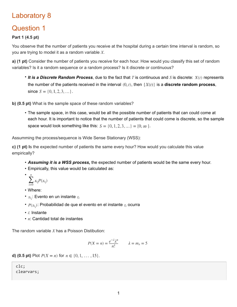
Laboratory 8
Question 1
Part 1 (4.5 pt)
You observe that the number of patients you receive at the hospital during a certain time interval is random, so
you are trying to model it as a random variable X.
a) (1 pt) Consider the number of patients you receive for each hour. How would you classify this set of random
variables? Is it a random sequence or a random process? Is it discrete or continuous?
• It is a Discrete Random Process, due to the fact that T is continuous and S is discrete:
the number of the patients received in the interval
, then
represents
is a discrete random process,
.
since
b) (0.5 pt) What is the sample space of these random variables?
• The sample space, in this case, would be all the possible number of patients that can could come at
each hour. It is important to notice that the number of patients that could come is discrete, so the sample
space would look something like this:
.
Assumming the process/sequence is Wide Sense Stationary (WSS):
c) (1 pt) Is the expected number of patients the same every hour? How would you calculate this value
empirically?
• Assuming it is a WSS process, the expected number of patients would be the same every hour.
• Empirically, this value would be calculated as:
•
• Where:
• : Evento en un instante
•
: Probabilidad de que el evento en el instante
• i: Instante
• n: Cantidad total de instantes
The random variable X has a Poisson Distibution:
d) (0.5 pt) Plot
for
clc;
clearvars;
1
ocurra
lmd=5;
mx=5;
N=16;
n=0:N-1;
P_X=(exp(-lmd)*lmd.^n)./(factorial(n));
figure;
bar(n,P_X);title("Poisson Distribution");grid on;
e) (1.5 pt) Use the function poissrnd(5,1,1000) to simulate the number of patients you receive each hour for
1000 hours. Using a bin for each number of patients, plot an histogram of the obtained vector and compare with
the result obtained in (d). Is it similar?
hrs=1000;
x=poissrnd(lmd,1,hrs); % using the function
P_X_alt=zeros(1,N); %defining a empty matrix
for k=1:N
P_X_alt(k)=double(sum(x==n(k)))/hrs;
end
figure;
bar(n,P_X_alt);title("Poisson Distribution 2");grid on;
2
P_X_alt
P_X_alt = 1×16
0.0070
0.0370
0.0880
0.1440
0.1720
0.1700
0.1400
0.1000
%otherwise
binEdges = [0.5 1.5 2.5 3.5 4.5 5.5 6.5 7.5 8.5 9.5 10.5 11.5 12.5 13.5 14.5 15.5 16.5];
[binCounts, binEdges] = histcounts(x, binEdges);
totalCounts = sum(binCounts);
pmf = binCounts/totalCounts;
% Plot the PMF
centers = (binEdges(2:end)+binEdges(1:end-1))/2;
figure;
stem(centers, pmf, 'filled', 'MarkerSize', 4);
xlabel("x"); ylabel("p(X<x)");
title("Probability Mass Function")
3
%figureSize = [500, 200]; % Width and height in pixels
%set(gcf, 'Position', [100, 100, figureSize]);
Part 2 (5.5 pt)
Recordings from any electrical sensor, like accelerometers, microphones, pressure sensors, etc, are subject
to thermal noise, generated by agitation of electrons inside a conductor. This noise can be modelled as a
continuous random process with a gaussian distribution.
Assume you are getting recordings from an accelerometer to estimate position. Once you digitalize the signal,
you get:
Where
is the true signal from the accelerometer and
a) (1 pt) How would you classify
continuous?
is the voltage from the noise.
? Is it a random sequence or a random process? Is it discrete or
• It is a Discrete Random Process, due to the fact that T is continuous and S is discrete:
, since digital thermal noise can take values
represents the digital thermal noise on some interval
ranging from the minimum to maximum reading limits wit an specific resolution (based on the device)
.
4
• It is important to remember that
is a digital signal, with discrete time and amplitude, so even if the
thermal noise is completely analog, and a continuous random process, the digital signal registered
from the accelerometer it is a different story.
The Probability Density Function of a gaussian distribution is:
For the recorded thermal noise,
b) (0.5 pt) If
pdf of
and
.
is Strict Sense Stationary, what is the probability density function of
? What would be the
?
Donde:
x: Las variables aleatorias (Rango de valores que puede tomar v[n]
c) (0.5 pt) Generate
for
using the function randn. Plot an histogram of the obtained data.
N2=10000;
n2=0:N2-1;
v=randn([1,N2]);
% hist=zeros(1,N2);
% for k=1:N2-1
%
hist(k)=double(sum(v==n2(k)))/N2;
% end
figure;
histogram(v,"Normalization","probability");title("Data Histogram");grid on;
5
d) (1 pt) Use the function [rx, lags] = xcorr(x,'biased') to generate the autocorrelation of
lags from 0 to 20 using stem. What do you observe?
[rv,lags]=xcorr(v,"biased");
figure;
stem(lags,rv);xlabel("Time in samples (n)");
ylabel("Cross-Correlation Amplitude");title("Autocorrelation v[n]");
grid on;xlim([0 20]);
6
. Plot it for
%We can observe that the maximum correlation it is obtained on sample 0 (with amplitude of 1),
%and then the correlation values range in amplitudes close to 0.
You try to use a low-pass filter
noise.
to recover the signal
e) (1 pt) Generate a FIR low pass filter with N = 50 and
sampling frequency. Filter
, but you want to know what happens with the
, where
generated in (d).
N_filt=50;
fs=1000;
fc=0.1*fs;
wc_nrm=fc/(fs/2);
[b,a]=fir1(N_filt,wc_nrm,"low");
figure;
sgtitle("FIR filter");
freqz(b,a,1000,fs);
7
is the cut frequency and
is the
f) (1.5 pt) Plot the histogram and the autocorrelation of the filtered signal, just as you did for
differences do you observe?
. What
v_filt=filter(b,a,v);
[rv_2,lags_2]=xcorr(v_filt,"biased");
figure;
histogram(v_filt,"Normalization","probability");title("Data Histogram (v_{filt})");grid on;
8
figure;
stem(lags_2,rv_2);xlabel("Time in samples (n)");
ylabel("Cross-Correlation Amplitude");title("Autocorrelation Filtered v[n]");
grid on;xlim([0 20]);
9
Question 2
You must read the paper “Using MATLAB for teaching transformations of random variables”, here is exposed
different classification for random variables transformations.
A. (3 pts) Implement an example of linear transformation for 1000 random variables:
• Gaussian distribution
• Uniform distribution
Plot the random variables and their pdf for the input and output of the transformation. Discuss the
characteristics of pdf in each case, you have to use equation 1 on the paper and explain the relationship
between the input and output.
%Assuming mean=0 and std=1:
N3=1000;
in_gd=randn([1,N3]);
in_ud=rand([1 N3]);
a=3;
b=5;
out_gd_lin=a*in_gd+b;
10
out_ud_lin=a*in_ud+b;
figure;
sgtitle("Linear Transformation");
subplot(221);
histogram(in_gd);title("PDF from Input Gaussian Distribution");
subplot(222);
histogram(out_gd_lin);title("PDF from Linear Output Gaussian Distribution");
subplot(223);
histogram(in_ud);title("PDF from Input Uniform Distribution");
subplot(224);
histogram(out_ud_lin);title("PDF from Linear Output Uniform Distribution");
B. (3 pts) Repeat item A for nonlinear transformation.
out_gd_nolin=exp(in_gd);
out_ud_nolin=exp(in_ud);
figure;
sgtitle("Non-Linear Transformation");
subplot(221);
histogram(in_gd);title("PDF from Input Gaussian Distribution");
subplot(222);
histogram(out_gd_nolin);title("PDF from Non-Linear Output Gaussian Distribution");
subplot(223);
histogram(in_ud);title("PDF from Input Uniform Distribution");
subplot(224);
11
histogram(out_ud_nolin);title("PDF from Non-Linear Output Uniform Distribution");
C. (3 pts) Repeat item A for non-monotone transformation. In this case, you have tou use equation 5.
out_gd_nomon=(in_gd).^2;
out_ud_nomon=(in_ud).^2;
figure;
sgtitle("Non-Linear Transformation");
subplot(221);
histogram(in_gd);title("PDF from Input Gaussian Distribution");
subplot(222);
histogram(out_gd_nomon);title("PDF from Non-Monotone Output Gaussian Distribution");
subplot(223);
histogram(in_ud);title("PDF from Input Uniform Distribution");
subplot(224);
histogram(out_ud_nomon);title("PDF from Non-Monotone Output Uniform Distribution");
12
D. (1 pt) What are the differences between monotone and non-monotone transformation?
13