Chapter one
1.
Introduction to Data Structures and Algorithms Analysis
A program is written in order to solve a problem. A solution to a problem actually consists of
two things:
 A way to organize the data
 Sequence of steps to solve the problem
The way data are organized in a computer’s memory is said to be Data Structure and the
sequence of computational steps to solve a problem is said to be an algorithm. Therefore, a
program is nothing but data structures plus algorithms.
1.1 Introduction to Data Structures
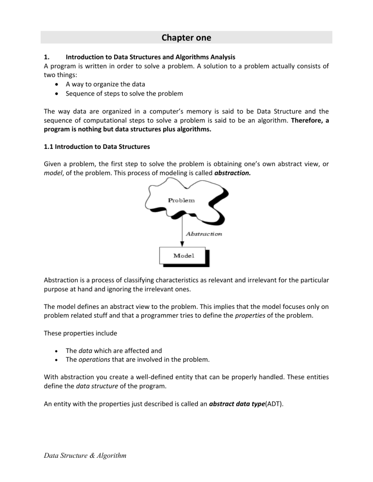
Given a problem, the first step to solve the problem is obtaining one’s own abstract view, or
model, of the problem. This process of modeling is called abstraction.
Abstraction is a process of classifying characteristics as relevant and irrelevant for the particular
purpose at hand and ignoring the irrelevant ones.
The model defines an abstract view to the problem. This implies that the model focuses only on
problem related stuff and that a programmer tries to define the properties of the problem.
These properties include


The data which are affected and
The operations that are involved in the problem.
With abstraction you create a well-defined entity that can be properly handled. These entities
define the data structure of the program.
An entity with the properties just described is called an abstract data type(ADT).
Data Structure & Algorithm
1.1.1. Why do we need data structures?
• Data structures allow us to achieve an important goal: component reuse; Once each data
structure has been implemented once, it can be used over and over
again in various applications.
Common data structures are
• Stacks
• Queues
• Lists
1.2.
• Trees
• Graphs
• Tables
Algorithms
An algorithm is a well-defined computational procedure that takes some value or a set
of values as input and produces some value or a set of values as output.
1.2.1. Properties of an algorithm
•
•
Finiteness: Algorithm must complete after a finite number of steps.
•
Sequence: Each step must have a unique defined preceding and succeeding step.
The first step (start step) and last step (halt step) must be clearly noted.
•
•
•
•
Correctness: It must compute correct answer for all possible legal inputs.
•
Efficiency: It must solve with the least amount of computational resources such as
time and space.
Definiteness: Each step must be clearly defined, having one and only one
interpretation. At each point in computation, one should be able to tell exactly what
happens next.
Language Independence: It must not depend on any one programming language.
Completeness: It must solve the problem completely.
Effectiveness: It must be possible to perform each step exactly and in a finite
amount of time.
1.2.2. Algorithm Analysis Concepts
Algorithm analysis refers to the process of determining the amount of computing time and
storage space required by different algorithms. In other words, it’s a process of predicting the
resource requirement of algorithms in a given environment.
In order to solve a problem, there are many possible algorithms. One has to be able to choose
the best algorithm for the problem at hand using some scientific method. To classify some data
structures and algorithms as good, we need precise ways of analyzing them in terms of
resource requirement. The main resources are:



Running Time
Memory Usage
Communication Bandwidth
Data Structure & Algorithm
Running time is usually treated as the most important since computational time is the most
precious resource in most problem domains.
However, it is difficult to use actual clock-time as a consistent measure of an algorithm’s
efficiency, because clock-time can vary based on many things. For example,




Specific processor speed
Current processor load
Specific data for a particular run of the program
o Input Size
o Input Properties
Operating Environment
Accordingly, we can analyze an algorithm according to the number of operations required,
rather than according to an absolute amount of time involved. This can show how an
algorithm’s efficiency changes according to the size of the input.
1.2.3. Complexity Analysis
Complexity Analysis is the systematic study of the cost of computation, measured either in time
units or in operations performed, or in the amount of storage space required.
The goal is to have a meaningful measure that permits comparison of algorithms independent
of operating platform.
There are two things to consider:
 Time Complexity: Determine the approximate number of operations required to solve a
problem of size n.
 Space Complexity: Determine the approximate memory required to solve a problem of
size n.
Complexity analysis involves two distinct phases:


Algorithm Analysis: Analysis of the algorithm or data structure to produce a function T
(n) that describes the algorithm in terms of the operations performed in order to
measure the complexity of the algorithm.
Order of Magnitude Analysis: Analysis of the function T (n) to determine the general
complexity category to which it belongs.
There is no generally accepted set of rules for algorithm analysis. However, an exact count of
operations is commonly used.
1.2.4. Analysis Rules:
2.
3.
We assume an arbitrary time unit.
Execution of one of the following operations takes time 1:
 Assignment Operation
Data Structure & Algorithm
 Single Input Operation
 Single Output Operation
 Single Boolean Operations
 Single Arithmetic Operations
 Function Return
4.
Running time of a selection statement (if, switch) is the time for the condition
evaluation + the maximum of the running times for the individual clauses in the
selection.
5.
Loops: Running time for a loop is equal to the running time for the statements inside the
loop * number of iterations.
The total running time of a statement inside a group of nested loops is the running time
of the statements multiplied by the product of the sizes of all the loops.
For nested loops, analyze inside out.
 Always assume that the loop executes the maximum number of iterations possible.
6.
Running time of a function call is 1 for setup + the time for any parameter calculations +
the time required for the execution of the function body.
Examples:
1. int count()
{
int k=0;
cout<< “Enter an integer”;
cin>>n;
for (i=1;i<=n;i++)
k=k+1;
return 0;
}
Time Units to Compute
------------------------------------------------1 for the assignment statement: int k=0
1 for the output statement.
1 for the input statement.
In the for loop:
1 assignment, n+1 tests, and n increments.
n loops of 2 units for an assignment, and an addition.
1 for the return statement.
------------------------------------------------------------------T (n) = 1+1+1+(1+n+1+n)+2n+1 = 4n+6 = O(n)
2. int total(int n)
{
int sum=0;
for (int i=1;i<=n;i++)
sum=sum+1;
return sum;
}
Time Units to Compute
Data Structure & Algorithm
------------------------------------------------1 for the assignment statement: int sum=0
In the for loop:
1 assignment, n+1 tests, and n increments.
n loops of 2 units for an assignment, and an addition.
1 for the return statement.
------------------------------------------------------------------T (n) = 1+ (1+n+1+n)+2n+1 = 4n+4 = O(n)
3. void func()
{
int x=0;
int i=1;
int j=1;
cout<< “Enter an Integer value”;
cin>>n;
while (i<=n)
{
x++;
i++;
}
while (j<n)
{
j++;
}
}
Time Units to Compute
------------------------------------------------1 for the first assignment statement: x=0;
1 for the second assignment statement: i=0;
1 for the third assignment statement: j=1;
1 for the output statement.
1 for the input statement.
In the first while loop:
n+1 tests
n loops of 2 units for the two increment (addition) operations
In the second while loop:
n tests
n-1 increments
------------------------------------------------------------------T (n) = 1+1+1+1+1+n+1+2n+n+n-1 = 5n+5 = O(n)
4. int sum (int n)
{
int partial_sum = 0;
for (int i = 1; i <= n; i++)
Data Structure & Algorithm
partial_sum = partial_sum +(i * i * i);
return partial_sum;
}
Time Units to Compute
------------------------------------------------1 for the assignment.
1 assignment, n+1 tests, and n increments.
n loops of 4 units for an assignment, an addition, and two multiplications.
1 for the return statement.
------------------------------------------------------------------T (n) = 1+(1+n+1+n)+4n+1 = 6n+4 = O(n)
1.2.4. Formal Approach to Analysis
In the above examples we have seen that analysis is a bit complex. However, it can be
simplified by using some formal approach in which case we can ignore initializations, loop
control, and book keeping.
For Loops: Formally
•
In general, a for loop translates to a summation. The index and bounds of the summation
are the same as the index and bounds of the for loop.
N
for (int i = 1; i <= N; i++) {
sum = sum+i;
}
i 1
1 
•
N
Suppose we count the number of additions that are done. There is 1 addition per iteration
of the loop, hence N additions in total.
Nested Loops: Formally
•
Nested for loops translate into multiple summations, one for each for loop.
for (int i = 1; i <= N; i++) {
for (int j = 1; j <= M; j++) {
sum = sum+i+j;
}
}
•
N
M
N
i 1
j 1
i 1
  2   2M
Again, count the number of additions. The outer summation is for the outer for loop.
Consecutive Statements: Formally
•
 2 MN
Add the running times of the separate blocks of your code
Data Structure & Algorithm
for (int i = 1; i <= N; i++) {
sum = sum+i;
}
for (int i = 1; i <= N; i++) {
for (int j = 1; j <= N; j++) {
sum = sum+i+j;
}
}
 N   N N 
2
1    2  N  2 N
 i 1   i 1 j 1 
Conditionals: Formally
•
If (test) s1 else s2: Compute the maximum of the running time for s1 and s2.
if (test == 1) {
N
for (int i = 1; i <= N; i++) {
 N
sum = sum+i;

max 
1,
}}
i 1
 i 1
else for (int i = 1; i <= N; i++) {
for (int j = 1; j <= N; j++) {
max N , 2 N 2
sum = sum+i+j;
}}




2


j 1

 2N 2
N

1.2.5. Measures of Times
In order to determine the running time of an algorithm it is possible to define three functions
Tbest(n), Tavg(n) and Tworst(n) as the best, the average and the worst case running time of the
algorithm respectively.
Average Case (Tavg): The amount of time the algorithm takes on an "average" set of inputs.
Worst Case (Tworst): The amount of time the algorithm takes on the worst possible set of inputs.
Best Case (Tbest): The amount of time the algorithm takes on the smallest possible set of inputs.
We are interested in the worst-case time, since it provides a bound for all input – this is called
the “Big-Oh” estimate.
1.2.6. Asymptotic Analysis
Asymptotic analysis is concerned with how the running time of an algorithm increases with the
size of the input in the limit increases without bound.
There are five notations used to describe a running time function. These are:



Big-Oh Notation (O)
Big-Omega Notation ()
Theta Notation ()
Data Structure & Algorithm


Little-o Notation (o)
Little-Omega Notation ()
 The Big-Oh Notation
Big-Oh notation is a way of comparing algorithms and is used for computing the complexity of
algorithms; i.e., the amount of time that it takes for computer program to run. It’s only
concerned with what happens for very a large value of n. Therefore only the largest term in the
expression (function) is needed. For example, if the number of operations in an algorithm is n2 –
n, n is insignificant compared to n2 for large values of n. Hence the n term is ignored. Of course,
for small values of n, it may be important. However, Big-Oh is mainly concerned with large
values of n.
Formal Definition: The function f(n) is O(g(n)) if there exist positive numbers c and K
such that f(n) ≤ c.g(n) for all n ≥ K.
Examples: The following points are facts that you can use for Big-Oh problems:





1<=n for all n>=1
n<=n2 for all n>=1
2n<=n! for all n>=4
log2n<=n for all n>=2
n<=nlog2n for all n>=2
1. f(n)=10n+5 and g(n)=n. Show that f(n) is O(g(n)).
To show that f(n) is O(g(n)) we must show that constants c and k such that
f(n) <=c.g(n) for all n>=k
Or 10n+5<=c.n for all n>=k
Try c=15. Then we need to show that 10n+5<=15n
Solving for n we get: 5<5n or 1<=n.
So f(n) =10n+5 <=15.g(n) for all n>=1.
(c=15,k=1).
2. f(n) = 3n2 +4n+1. Show that f(n)=O(n2).
Data Structure & Algorithm
4n <=4n2 for all n>=1 and 1<=n2 for all n>=1
3n2 +4n+1<=3n2+4n2+n2 for all n>=1
<=8n2 for all n>=1
So we have shown that f(n)<=8n2 for all n>=1
Therefore, f (n) is O(n2) (c=8,k=1)
Typical Orders
Here is a table of some typical cases. This uses logarithms to base 2, but these are simply
proportional to logarithms in other base.
N
O(1)
O(log n)
O(n)
O(n log n)
O(n2)
O(n3)
1
1
1
1
1
1
1
2
1
1
2
2
4
8
4
1
2
4
8
16
64
8
1
3
8
24
64
512
16
1
4
16
64
256
4,096
1024
1
10
1,024
10,240
1,048,576
1,073,741,824
Demonstrating that a function f(n) is big-O of a function g(n) requires that we find specific
constants c and k for which the inequality holds (and show that the inequality does in fact
hold).
Big-O expresses an upper bound on the growth rate of a function, for sufficiently large values of
n.
An upper bound is the best algorithmic solution that has been found for a problem.
“ What is the best that we know we can do?”
Exercice:
f(n) = (3/2)n2+(5/2)n-3
Show that f(n)= O(n2)
Data Structure & Algorithm
In simple words, f (n) =O(g(n)) means that the growth rate of f(n) is less than or equal to g(n).
Big-OTheorems
For all the following theorems, assume that f(n) is a function of n and that k is an arbitrary
constant.
Theorem 1: k is O(1)
Theorem 2: A polynomial is O(the term containing the highest power of n).
Polynomial’s growth rate is determined by the leading term

If f(n) is a polynomial of degree d, then f(n) is O(nd)
In general, f(n) is big-O of the dominant term of f(n).
Theorem 3: k*f(n) is O(f(n))
Constant factors may be ignored
E.g. f(n) =7n4+3n2+5n+1000 is O(n4)
Theorem 4(Transitivity): If f(n) is O(g(n))and g(n) is O(h(n)), then f(n) is O(h(n)).
 Big-Omega Notation
Just as O-notation provides an asymptotic upper bound on a function,  notation provides an
asymptotic lower bound.
Formal Definition: A function f(n) is ( g (n)) if there exist constants c and k ∊ℛ+ such that
f(n) >=c. g(n) for all n>=k.
f(n)=( g (n)) means that f(n) is greater than or equal to some constant multiple of g(n) for all
values of n greater than or equal to some k.
Example: If f(n) =n2, then f(n)= ( n)
In simple terms, f(n)=( g (n)) means that the growth rate of f(n) is greater that or equal to g(n).
Data Structure & Algorithm
 Theta Notation
A function f (n) belongs to the set of  (g(n)) if there exist positive constants c1 and c2 such that
it can be sandwiched between c1.g(n) and c2.g(n), for sufficiently large values of n.
Formal Definition: A function f (n) is  (g(n)) if it is both O( g(n)) and  ( g(n)). In other words,
there exist constants c1, c2, and k >0 such that c1.g (n)<=f(n)<=c2. g(n) for all n >= k
If f(n)=  (g(n)), then g(n) is an asymptotically tight bound for f(n).
In simple terms, f(n)=  (g(n)) means that f(n) and g(n) have the same rate of growth.
Example:
1. If f(n)=2n+1, then f(n) =  (n)
2. f(n) =2n2 then
f(n)=O(n4)
f(n)=O(n3)
f(n)=O(n2)
All these are technically correct, but the last expression is the best and tight one. Since 2n2 and n2
have the same growth rate, it can be written as f(n)= (n2).
 Little-o Notation
Big-Oh notation may or may not be asymptotically tight, for example:
2n2 = O(n2)
=O(n3)
f(n)=o(g(n)) means for all c>0 there exists some k>0 such that f(n)<c.g(n) for all n>=k.
Informally, f(n)=o(g(n)) means f(n) becomes insignificant relative to g(n) as n approaches
infinity.
Example: f(n)=3n+4 is o(n2)
In simple terms, f(n) has less growth rate compared to g(n).
g(n)= 2n2 g(n) =o(n3), O(n2), g(n) is not o(n2).
Data Structure & Algorithm
 Little-Omega ( notation)
Little-omega () notation is to big-omega () notation as little-o notation is to Big-Oh notation.
We use  notation to denote a lower bound that is not asymptotically tight.
Formal Definition: f(n)=  (g(n)) if there exists a constant no>0 such that 0<= c. g(n)<f(n) for
all n>=k.
Example: 2n2=(n) but it’s not  (n2).
Data Structure & Algorithm