Problem Set 1: Sketch of Solutions
Information Economics (Ec 515)
·
George Georgiadis
Problem 1.
Consider the following “portfolio choice” problem. The investor has initial wealth w and utility u ( x ) =
ln ( x ). There is a safe asset (such as a US government bond) that has net real return of zero. There is also a
risky asset with a random net return that has only two possible returns, R1 with probability q and R0 with
probability 1
q. Let A be the amount invested in the risky asset, so that w
A is invested in the safe asset.
1. Find A as a function of w. Does the investor put more or less of his portfolio into the risky asset as his
wealth increases?
2. Another investor has the utility function u ( x ) =
e
x.
How does her investment in the risky asset
change with wealth?
3. Find the coefficients of absolute risk aversion r ( x ) =
u00 ( x )
u0 ( x )
for the two investors. How do they
depend on wealth? How does this account for the qualitative difference in the answers you obtain in
parts (1) and (2)?
Solution of Problem 1:
Firstly, let’s set up the problem:
max {q u ((1 + R1 ) A + w−A) + (1
A2[0,w]
q) u ((1 + R0 ) A + w−A)}
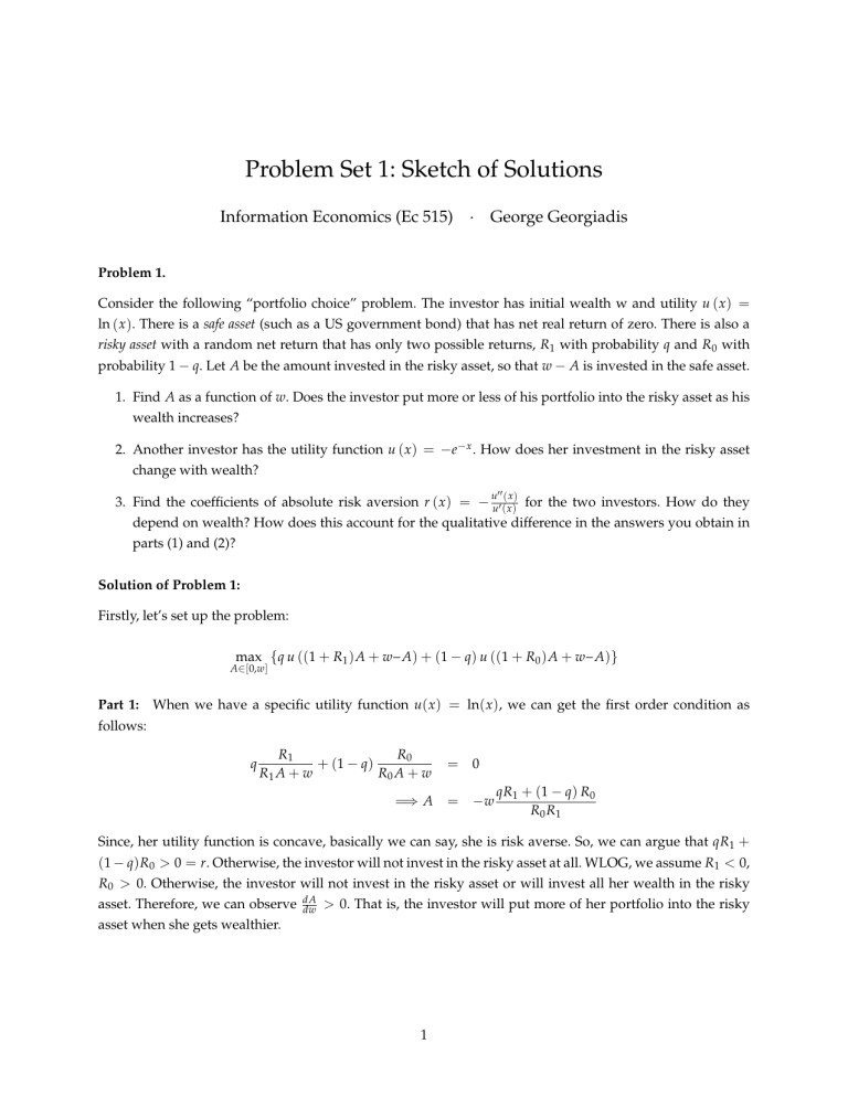
Part 1: When we have a specific utility function u( x ) = ln( x ), we can get the first order condition as
follows:
q
R1
+ (1
R1 A + w
q)
R0
R0 A + w
= 0
=) A =
w
qR1 + (1 q) R0
R0 R1
Since, her utility function is concave, basically we can say, she is risk averse. So, we can argue that qR1 +
(1 q) R0 > 0 = r. Otherwise, the investor will not invest in the risky asset at all. WLOG, we assume R1 < 0,
R0 > 0. Otherwise, the investor will not invest in the risky asset or will invest all her wealth in the risky
asset. Therefore, we can observe dA
dw > 0. That is, the investor will put more of her portfolio into the risky
asset when she gets wealthier.
1
Part 2:
From the first order condition,
R1 qe
( R1 A + w )
+ R0 (1
q)e
( R0 A + w )
= 0
1
=) A =
Observe that
dA
dw
R0
R1
ln

R0 (1 q )
R1 q
= 0 ; that is, her investment in the risky asset doesn’t change with wealth.
Part 3: For u( x ) = ln( x ), we have u0 ( x ) = 1x and u00 ( x ) = x12 . So r ( x ) = 1x ; i.e., as x gets bigger, r ( x ) gets
smaller, and so the wealthier the investor is, the less risk averse she is. Therefore, she will put more wealth
into the risky asset.
For u( x ) =
e
x,
we have u0 ( x ) = e
x
and u00 ( x ) =
e
x.
So r ( x ) = 1. Therefore, the amount that the
investor allocates to the risky asset is independent of her wealth.
Problem 2.
You have an opportunity to place a bet on the outcome of an upcoming race involving a certain female horse
named Bayes: if you bet x dollars and Bayes wins, you will have w0 + x, while if she loses you will have
w0
x, where w0 is your initial wealth.
1. Suppose that you believe the horse will win with probability p and that your utility for wealth w is
ln (w). Find your optimal bet as a function of p and w0 .
2. You know little about horse racing, only that racehorses are either winners or average, that winners
win 90% of their races, and that average horses win only 10% of their races. After all the buzz you’ve
been hearing, you are 90% sure that Bayes is a winner. What fraction of your wealth do you plan to
bet?
3. As you approach the betting window at the track, you happen to run into your uncle. He knows rather
a lot about horse racing: he correctly identifies a horse’s true quality 95% of the time. You relay your
excitement about Bayes. “Don’t believe the hype,” he states. “That Bayes mare is only an average
horse.” What do you bet now (assume that the rules of the track permit you to receive money only if
the horse wins)?
Solution of Problem 2:
Part 1:
The expected utility from betting x is:
EU ( x ) = p ln(w0 + x ) + (1
p) ln(w0
x)
Your objective is to choose x to maximize your expected utility. The first order condition w.r.t x is
p
w0 + x
x⇤
1 p
w0 x
w0 (2p 1)
=
=
2
Part 2:
Your probability that Bayes will win can be determined as follows:
p = 0.9 ⇥ 0.9 + 0.1 ⇥ 0.1 = 0.82
Therefore, using the formula from part 1, we obtain x ⇤ = w0 (2 ⇥ 0.82
Part 3:
1) = 0.64w0
Let q denote the true type of Bayes. “q = 1” means Bayes is a winner, “q = 0” means Bayes is
average. Let s denote the signal from your uncle. “s = 1” means uncle asserts Bayes is a winner, and “s = 0”
means uncle asserts Bayes is average. The uncle’s signal is accurate 95% of the time, i.e.,
Pr(s = 1|q = 1) = Pr(s = 0|q = 0) = 0.95
Therefore, the updated belief is
Pr(q = 1|s = 0)
=
=
=
=
Pr(q = 1, s = 0)
Pr(s = 0)
Pr(s = 0|q = 1) ⇥ Pr(q = 1)
Pr(s = 0, q = 1) + Pr(s = 0, q = 0)
Pr(s = 0|q = 1) ⇥ Pr(q = 1)
Pr(s = 0|q = 1) ⇥ Pr(q = 1) + Pr(s = 0|q = 0) ⇥ Pr(q = 0)
0.05 ⇥ 0.9
= 0.32
0.05 ⇥ 0.9 + 0.95 ⇥ 0.1
Using the formula from part 1 again, we obtain x ⇤ =
0.357w0 < 0. You would like to bet against Bayes,
but this is not allowed, so the optimal choice is to bet nothing.
Problem 3.
If an individual devotes a units of effort in preventative care, then the probability of an accident is 1
a
(thus, effort can only assume values in [0, 1]). Each individual is an expected utility maximizer with utility
function p ln ( x ) + (1−p) ln (y)
a2 , where p is the probability of an accident, x is wealth if there is an
accident, and y is wealth if there is no accident. If there is no insurance, then x = 50, while y = 150.
1. Suppose first there is no market for insurance. What level of a would the typical individual choose?
What would her expected utility be?
2. Assume that a is verifiable. What relationship do you expect to prevail between x and y in a competitive insurance market? What relationship do you then expect to prevail between x and a?
3. Derive the value of a, x and y that maximize the typical customer’s expected utility. What is the value
of this maximized expected utility?
4. Suppose that a is not verifiable. What would happen (i.e., what would the level of a and expected
utility be) if the same contract (i.e., same x and y values) as in (3) were offered by competitive firms?
Do you expect this would be an equilibrium?
5. Under the non-verifiability assumption, what relationship must prevail between x, y, and a? Use this
relationship along with the assumption of perfect competition to derive a relationship between x and
3
a that contracts offered by insurers must have. Finally, find the level of a that maximizes the expected
utility of the typical consumer, and find that level of expected utility.
6. Summarize your answers by ranking the levels of a and the expected utilities for each of the cases in
(1), (3), (4) and (5). What do you notice?
Solution of Problem 3:
Part 1:
The consumer solves
n
max (1
a
The first order condition w.r.t a is
Part 2:
o
ln(50) + ln(150) = 2a, which in turn implies that a =
ln(3)
2
' 0.55.
Without moral hazard, the consumer will be fully insured, so x = y. Perfect competition implies
that firms will make 0 profits, so x = y = (1
Part 3:
a2
a) ln(50) + a ln(150)
a)50 + a150 = 50 + 100a.
Using the answer from part 2, we solve
n
o
max ln(50 + 100a)−a2
a
It follows from the first order condition that a = 12 , and so x = 50 + 100a = 100
Part 4: if x = y = 100 and a is not verfiable, then the consumer will set a = 0. Since x = 100 from above,
firms lose money (they get 50 and pay out 100 always), so this cannot be an equilibrium.
Part 5:
Each firm solves
max
(1
a,x,y
s.t.
a) ln( x ) + a ln(y)
a2
(1−a) x + ay = (1−a)50 + a150
a 2 arg max (1
y
x
The first order condition for (IC) is ln
and so the problem simplifies to
a) ln( x ) + a ln(y)
a2
(IC)
= 2a, so y = e2a x. Plugging this into (ZP) yields x =
⇢
✓
max a2 + ln
a
(ZP)
50 + 100a
1 + a (e2a 1)
After some algebra, the first order condition simplifies to 2(2a3
50+100a
,
1+ a(e2a 1)
◆
a2
a) =
e2a 3
.
e2a 1
Using a software package
such as Matlab, one obtains a ' 0.37, and plugging back we get the expected utility 4.26.
Part 6:
The first best in (c) gives the consumer the highest expected utility with a = 0.5, the second best in
(e) yields the second highest expected utility with a = 0.37, and no insurance has the lowest expected utility
with a = 0.55. Hence, we notice that, consumers will have a lower expected utility without insurance, even
though they have devoted a higher effort a to prevent accidence.
4
Problem 4.
An agent can work for a principal. The agent’s effort, a affects current profits, q1 = a + # q1 , and future
profits, q2 = a + # q2 , where # qt are random shocks, and they are i.i.d with normal distribution N (0, sq2 ).
The agent retires at the end of the first period, and his compensation cannot be based on q2 . However, his
compensation can depend on the stock price P = 2a + # P , where # P ⇠ N (0, sP2 ). The agent’s utility function
is exponential and equal to
h
i
2
h t c a2
e
where t is the agent’s income, while his reservation utility is t̄.1 The principal chooses the agent’s compensation contract t = w + f q1 + sP to maximize her expected profit, while accounting for the agent’s IR and
IC constraints.
1. Derive the optimal compensation contract t = w + f q1 + sP.
2. Discuss how it depends on sP2 and on its relation with sq2 . Offer some intuition?
Solution of Problem 4:
The program for this problem is the following,
max E (q1 + q2
a,w, f ,s
t)
subject to
E
✓
e
h
i
2 ◆
h t c a2
,
e
ht
arg max E
(1)
✓
a
2
t
= w + f q1 + sP
max 2a
a,w, f ,s
b
a
e
h
i
2 ◆
h t c a2
(2)
(3)
(w + f a + 2sa)
subject to
⌘ c
h⇣ 2 2
f sq + s2 sP2 + 2s f sqP
a2 t
2
2
⌘ c
h⇣ 2 2
b
a 2 arg max w + f b
a + 2sb
a
f sq + s2 sP2 + 2s f sqP
a2 .
2
2
b
a
w + f a + 2sa
We can apply the first-order approach and substitute the first order condition
a=
f + 2s
c
for the incentive compatibility constraint. Introducing this efficient level of effort and substituting the out1 Reservation
utility t̄ means that the agent’s IR constraint requires that E
5
e

2
h t c a2 )
e
h t̄ .
side opportunity level plus the risk premium plus the cost of effort for the wage, we obtain
max 2
f ,s
f + 2s
c
⌘
h⇣ 2 2
f sq + s2 sP2 + 2s f sqP
2
( f + 2s)2
2c
t.
The first order conditions with respect to f and s are respectively
4
c
2
c
⇣
⌘ f ⇤ + 2s⇤
h f ⇤ sq2 + s⇤ sqP
c
⇣
⌘
f ⇤ + 2s⇤
⇤ 2
⇤
h s sP + f sqP
2
c
= 0
= 0.
After some rewriting, the equations become
f⇤
f
⇤
=
=
2
s⇤ (2 + hcsqP )
1 + hcsq2
2
s ⇤ (2 +
1+
hcsP2
2 )
hcsqP
2
,
and we finally find
f⇤
s⇤
=
=
2sq2 +
sP2
2
sP2
2sqP
2sqP +
2sq2
2sq2 +
sP2
2
2sqP +
hc
2 2
2 ( sP sq
2 )
sqP
sqP
hc
2 2
2 ( sP sq
2 )
sqP
.
Problem 5.
Two agents can work for a principal. The output of agent i (i = 1, 2), is qi = ai + # i , where ai is agent i’s
effort level and # i is a random shock. The # i ’s are independent of each other and normally distributed with
mean 0 and variance s2 . In addition to choosing a2 , agent 2 can engage in a second activity b2 . This activity
does not affect output directly, but rather reduces the effort cost of agent 1. The interpretation is that agent
2 can help agent 1 (but not the other way around). The effort cost functions of the agents are
y1 ( a1 , b2 ) =
1
(a
2 1
and
y2 ( a2 , b2 ) =
b2 )2
1 2
a + b22 .
2 2
Agent 1 chooses her effort level a1 only after she has observed the level of help b2 . Agent i’s utility function
is exponential and equal to
e[
h (wi yi ( ai ,b2 ))]
where wi is the agent’s income. The agent’s reservation utility is
1, which corresponds to a reservation
wage of 0. The principal is risk neutral and is restricted to linear incentive schemes. The incentive scheme
for agent i is
wi = z i + v i q i + u i q j
6
1. Assume that a1 , a2 , and b2 are observable. Solve the principal’s problem by maximizing the total expected surplus with respect to a1 , a2 , and b2 . Explain intuitively why a1 > a2 .
2. Assume from now on that a1 , a2 , and b2 are not observable. Solve again the principal’s problem. Explain intuitively why u1 = 0.
3. Assume that the principal cannot distinguish whether a unit of output was produced by agent 1 or
agent 2. The agents can thus engage in arbitrage, claiming that all output was produced by one of them.
Assume that they will do so whenever it increases the sum of their wages. Explain why the incentive
scheme in part 2 above leads to arbitrage. What additional constraint does arbitrage impose on the
principal’s problem? Solve this problem, and explain intuitively why u1 > 0.
Solution of Problem 5:
Part 1: First-Best Outcome
The principal can observe a1 , a2 , and b2 and maximizes the total expected
surplus
1h
( a1
2
max ES = a1 + a2
a1 ,a2 ,b2
The first order conditions yield
1
b2 )
= 0
a2
= 0
b2
2b2
= 0.
a1
=
a2
=
b2
=
( a1
1
a1
i
b2 )2 + a22 + 2b22 + hV (w) .
Solving these equations we obtain
3
2
1
1
.
2
Note that a1 > a2 , that is, agent 1 exerts more effort in activity a1 than agent 2 in a2 since at an interior
solution where agent 2 exerts positive effort in activity b2 agent 1’s marginal cost is lower.
Part 2: Unobservable Effort and Linear Contracts The principal’s problem is to solve
max Ep = a1 (1
v1
u2 ) + a2 (1
v2
u1 )
z1
z2
subject to
h 2 2
1
s (v1 + u21 )
(a
b2 )2
2
2 1
h 2 2
1 2
z2 + v2 a2 + u2 a1
s (v2 + u22 )
a
b22
2
2 2
z1 + v1 a1 + u1 a2
7
0
(4)
0
(5)
and
a1
a2 , b2
⇢
1
(a
b2 )2
2 1
1 2
a
b22
2 2
h 2 2
s (v1 + u21 )
2
h 2 2
s (v2 + u22 )
2
2 arg max z1 + v1 a1 + u1 a2
⇢
2 arg max z2 + v2 a2 + u2 a1
(6)
(7)
From the incentive compatibility constraints we can obtain the best-response functions of the two agents.
Note that agent 1 chooses his effort level a1 after he has observed the level of help b2 . Agent 1’s first order
condition for a1 yields
a1 = v1 + b2 .
(8)
Hence we can rewrite the maximization problem for agent 2 as
max z2 + v2 a2 + u2 (v1 + b2 )
a2 ,b2
h 2 2
s (v2 + u22 )
2
1 2
a
2 2
b22 .
Solving the resulting system of equations we obtain
a1
= v1 +
a2
= v2
u2
=
.
2
b2
u2
2
Substituting these equations as well as the binding participation constraints into the principal’s problem we
are left with the following unconstrained maximization problem
max
v1 ,v2 ,u1 ,u2
(
u2
v1 +
+ v2
2
h 2 2
s (v1 + u21 + v22 + u22 )
2
1
2
v21
+ v22
u2
+ 2
2
!)
.
The first order conditions are
1
hs2 v1
v1
= 0
1
2
v2
= 0
hs2 u1
u2
hs2 u2
2
= 0
1
2
hs v2
= 0
which yield
v1
=
v2
=
u1
=
u2
=
1
1 + hs2
1
1 + hs2
0
1
.
1 + 2hs2
Note that even though v1 = v2 we have a1 > a2 as before in the first-best solution. This is the result of a
positive u2 . Agent 2 has to receive a share of agent 1’s output in order to incentivize him to help agent 2. On
8
the other hand, agent 1 does not receive a share of agent 2’s output (u1 = 0) since he cannot help agent 1 and
making his wage contingent on agent 1’s output only introduces costly variance into his wage payment.
Part 3: Arbitrage
The optimal payment scheme proposed above is not robust to arbitrage since v1 = v2 ,
yet u2 > u1 . As a result in order to increase the sum of their wages the agents will always claim that all
output was produced by agent 1 (since agent 2 receives a share of his output). In order to prevent arbitrage
the principal has to ensure that for the sum of wages the marginal return to both outputs is the same so that
the agents are indifferent between claiming that outputs are produced by one or the other:
v1 + u2 = v2 + u1 .
The principal now maximizes
u2
max v1 +
+ v2
v1 ,v2 ,u1 ,u2
2
h 2 2
s (v1 + u21 + v22 + u22 )
2
1
2
v21
+ v22
u2
+ 2
2
!
subject to the new arbitrage constraint. Eliminating u1 from the maximand using the above constraint, results in the first order conditions for v1 , v2 and u2 being
(1 + 2hs2 )v1
hs2 v2 + hs2 u2
2
2
hs v1 + (1 + 2hs )v2
2hs2 v1
2
= 1
hs u2
= 1
2hs2 v2 + (1 + 4hs2 )u2
= 1
which can be solved to obtain
7h 2 s4 + 6hs2 + 1
(8h 2 s4 + 7hs2 + 1)(hs2 + 1)
v1
=
v2
=
u1
=
hs2 + 1
8h 2 s4 + 7hs2 + 1
u2
=
3hs2 + 1
.
8h 2 s4 + 7hs2 + 1
9h 2 s4 + 8hs2 + 1
+ 7hs2 + 1)(hs2 + 1)
(8h 2 s4
First note that v1 < v2 and u1 < u2 , so agent 1 receives a lower wage payment scheme in equilibrium.
However, in contrast to the previous case where we ruled out arbitrage, we have u1 > 0. In order to satisfy
the arbitrage constraint the principal has to raise v2 and u1 even though the latter only introduces additional
noise into the wage payment to the agents.
9