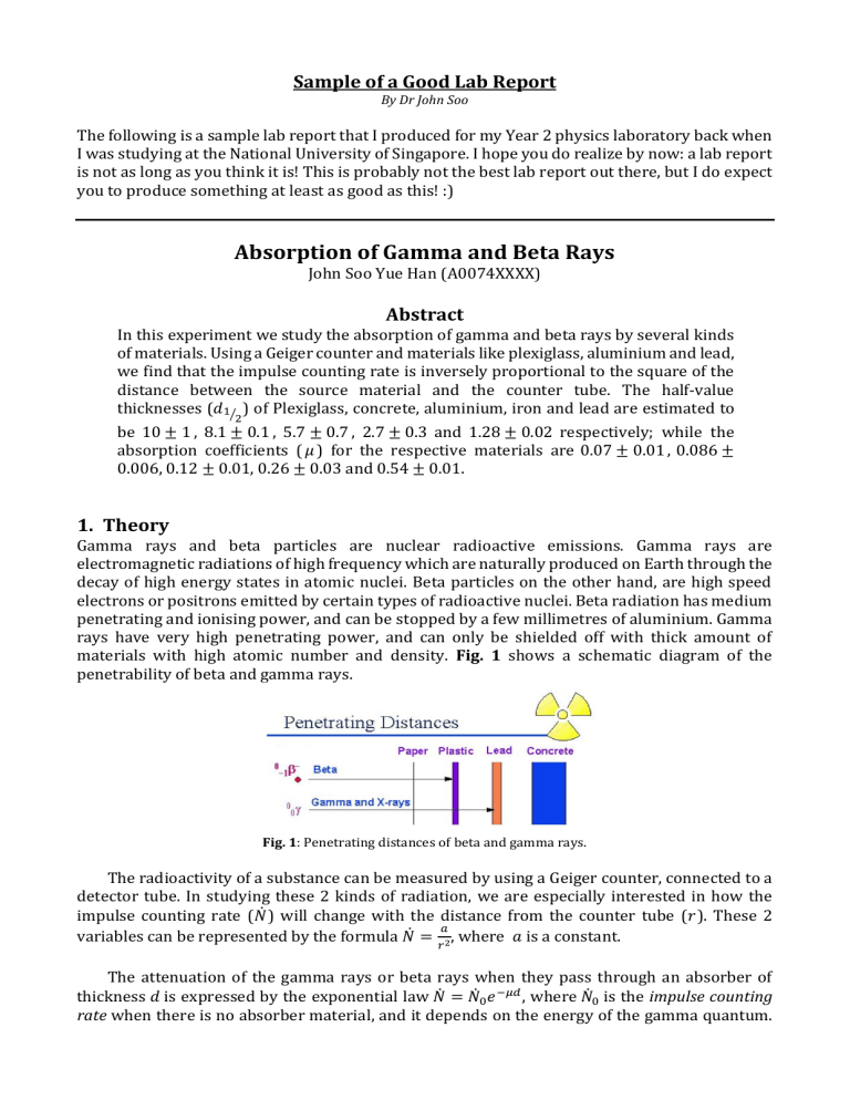
Sample of a Good Lab Report By Dr John Soo The following is a sample lab report that I produced for my Year 2 physics laboratory back when I was studying at the National University of Singapore. I hope you do realize by now: a lab report is not as long as you think it is! This is probably not the best lab report out there, but I do expect you to produce something at least as good as this! :) Absorption of Gamma and Beta Rays John Soo Yue Han (A0074XXXX) Abstract In this experiment we study the absorption of gamma and beta rays by several kinds of materials. Using a Geiger counter and materials like plexiglass, aluminium and lead, we find that the impulse counting rate is inversely proportional to the square of the distance between the source material and the counter tube. The half-value thicknesses (𝑑1⁄ ) of Plexiglass, concrete, aluminium, iron and lead are estimated to 2 be 10 ± 1 , 8.1 ± 0.1 , 5.7 ± 0.7 , 2.7 ± 0.3 and 1.28 ± 0.02 respectively; while the absorption coefficients ( 𝜇 ) for the respective materials are 0.07 ± 0.01 , 0.086 ± 0.006, 0.12 ± 0.01, 0.26 ± 0.03 and 0.54 ± 0.01. 1. Theory Gamma rays and beta particles are nuclear radioactive emissions. Gamma rays are electromagnetic radiations of high frequency which are naturally produced on Earth through the decay of high energy states in atomic nuclei. Beta particles on the other hand, are high speed electrons or positrons emitted by certain types of radioactive nuclei. Beta radiation has medium penetrating and ionising power, and can be stopped by a few millimetres of aluminium. Gamma rays have very high penetrating power, and can only be shielded off with thick amount of materials with high atomic number and density. Fig. 1 shows a schematic diagram of the penetrability of beta and gamma rays. Fig. 1: Penetrating distances of beta and gamma rays. The radioactivity of a substance can be measured by using a Geiger counter, connected to a detector tube. In studying these 2 kinds of radiation, we are especially interested in how the impulse counting rate (𝑁̇ ) will change with the distance from the counter tube (𝑟). These 2 𝑎 variables can be represented by the formula 𝑁̇ = 𝑟 2, where 𝑎 is a constant. The attenuation of the gamma rays or beta rays when they pass through an absorber of thickness 𝑑 is expressed by the exponential law 𝑁̇ = 𝑁̇0 𝑒 −𝜇𝑑 , where 𝑁̇0 is the impulse counting rate when there is no absorber material, and it depends on the energy of the gamma quantum. The variable 𝜇 is the absorption coefficient of a certain material, which is proportional to the number of electrons in the shell per unit volume, or approximately proportional to the density (𝜌) of the material. With this value, we could obtain the half-value thickness of a material (𝑑1⁄ ), 2 which is the thickness at which the impulse counting rate is reduced by half. This value is ln 2 represented by the equation 𝑑1/2 = 𝜇 . The aim of this experiment is to understand the interaction of radiation and matter, and the application to radiation detecting and shielding. In this experiment, we will find a. The relationship between the impulse counting rate and the distance between the source and the counter tube; and b. The half-value thickness (𝑑1⁄ ) and the absorption coefficient (𝜇) of Plexiglass, concrete, aluminium, iron and lead. 2 2. Experiment Fig. 2: Experimental setup for the absorption of gamma and beta rays. The apparatus is set up as shown in Fig. 2. The Geiger tube detector is mounted on a holder, and is made to face the radioactive source Cobalt-60 (60C) directly. The experiment is started with a background count for one minute, in which the counts are accounted by the cosmic rays and radioactive materials present in the ground and the building. This count is denoted by 𝑁̇𝐵 . For part A, the source is placed 4 cm away from the detector. The counter is then set to measure the amount of counts received in one minute (𝑁̇). A total of 6 readings are taken, and the average reading is calculated. The experiment is repeated for distances 5 cm, 6 cm, 7 cm, 8 cm and 9 cm. A linear least-squares-fit and a graph of ln(𝑁̇ − 𝑁̇𝐵 ) against ln 𝑟 is plotted, and the inverse square law is to be verified. In Part B, the experiment is first started by testing the amount of aluminum absorbers required to shield off the beta rays from being counted by the tube detector. This is done by inserting sheets of aluminium between the detector and the source, measure the count rate, and slowly increasing the number of sheets and remeasure until the count rate reaches a fairly constant value. The thickness of a block of Plexiglass is measured using a micrometer screw gauge, and it is placed together with the amount of aluminium sheets required to shield the beta rays earlier, in between the detector and the 60C source, which are 4 cm away from each other. The count rate for one minute is measured. The thickness of Plexiglass is slowly increased by inserting a few more blocks, and the count rate per minute is measured again each time. The experiment is repeated for blocks of concrete, aluminium, iron and lead. For each measurement, 6 readings are taken, and the average is calculated. A linear least-squares-fit and a graph of ln(𝑁̇ − 𝑁̇𝐵 ) against 𝑑 is plotted, the absorption coefficient 𝜇 and half-value thickness 𝑑1⁄ for 2 each material is calculated. 3. Results PART A The data collected for this experiment are attached in the Appendix. Based on the tables shown, the background count 𝑁̇𝐵 is calculated to be 31 ± 4 counts per minute. With the background count measured, the graph of ln(𝑁̇ − 𝑁̇𝐵 ) against ln 𝑟 is plotted and is shown in Fig. 3 below. Fig. 3: Graph of ln(𝑁̇– 𝑁̇𝐵 ) against ln 𝑟. 𝑎 Modifying the equation 𝑁̇ = 𝑟 2, we have ln 𝑁̇ = −2 ln 𝑟 + ln 𝑎, which is the equation of the line plotted. Fig. 3 shows a gradient of −𝟏. 𝟕 ± 𝟎. 𝟏, a 𝑦-intercept of 𝟖. 𝟐 ± 𝟎. 𝟐, and a correlation coefficient of 0.9833. This shows that there is quite strong positive correlation between both the variables. Comparing with the equation derived, the gradient of the graph is equal to the theoretical value -2 within 15% experimental uncertainty. PART B As per the previous part, the data collected are attached in the appendix for reference. From the beta particle shielding test, it shows that when we use aluminium sheets of thicknesses between 0.110 cm to 0.750 cm, the count rate is quite constant, and the count rate decreases drastically when the thickness of 0.925 cm is used. Therefore we made use of aluminium sheets of thickness 0.750 cm to shield the beta particles in the next few parts of the experiment. Modifying the equation 𝑁̇ = 𝑁̇0 𝑒 −𝜇𝑑 to express it as ln 𝑁̇ = −𝜇𝑑 + ln 𝑁̇0 , we see that the term −𝜇 is the gradient of a graph of ln 𝑁̇ against 𝑑 . The graphs for Plexiglass, concrete, aluminium, iron and lead are plotted as shown in Figs. 4 to 8. Fig. 4: Graph of ln(𝑁̇– 𝑁̇𝐵 ) against the thickness of plexiglass. Fig. 5: Graph of ln(𝑁̇– 𝑁̇𝐵 ) against the thickness of concret. Fig. 6: Graph of ln(𝑁̇– 𝑁̇𝐵 ) against the thickness of aluminium. Fig. 7: Graph of ln(𝑁̇– 𝑁̇𝐵 ) against the thickness of iron. Fig. 8: Graph of ln(𝑁̇– 𝑁̇𝐵 ) against the thickness of lead. We further summarise all the graphs shown earlier in Fig. 9 below. Fig. 9: A summary graph of ln(𝑁̇– 𝑁̇𝐵 ) against the thicknesses of the materials used in this experiment. The data collected from all the graphs in part B is summarized in Table 1. Material Plexiglass Concrete Aluminium Iron Lead Gradient, 𝒎 (cm-1) −0.07 ± 0.01 −0.086 ± 0.006 −0.12 ± 0.01 −0.26 ± 0.03 −0.54 ± 0.01 𝒚-intercept, 𝒄 5.79 ± 0.02 5.74 ± 0.02 5.75 ± 0.03 5.70 ± 0.07 5.80 ± 0.02 Correlation Coefficient, 𝒓 0.9234 0.9784 0.9493 0.9374 0.9987 Table 1: Data obtained from graphs plotted as shown in Figs. 4 to 8. From the data obtained above, we see that every graph has a correlation coefficient of at least 0.9200 and above. This shows that there is quite strong positive correlation between the variables, and the equation is well verified. Using the fact that the gradient 𝑚 = −𝜇, and 𝑑1⁄ = ln 2 𝜇 2 , we thus summarize our final values of absorption coefficients and half-value thicknesses together with their percentage discrepancies in Table 2 below. Material Plexiglass Concrete Aluminium Iron Lead Absorption Coefficient, 𝝁 (cm-1) 0.07 ± 0.01 0.086 ± 0.006 0.12 ± 0.01 0.26 ± 0.03 0.54 ± 0.01 Discr. Half-value Thickness, 𝒅𝟏⁄ (cm) Discr. 10 ± 1 8.1 ± 0.1 5.7 ± 0.7 2.7 ± 0.3 1.28 ± 0.02 7.9% 44.1% 23.9% 52.2% 14.0% 7.4% 30.7% 18.9% 34.3% 12.4% 𝟐 Table 2: Calculated values of the absorption coefficient and half-value thickness for the respective materials. 4. Discussion The errors for the measurements taken for a dependent variable y is based on the formula of propagation of errors, 2 2 2 𝜕𝑦 𝜕𝑦 𝜕𝑦 𝛿𝑦 = √( 𝛿𝑥 ) + ( 𝛿𝑥 ) + ⋯ + ( 𝛿𝑥 ) 𝜕𝑥1 1 𝜕𝑥2 2 𝜕𝑥𝑛 𝑛 where 1,2, … , 𝑛 denote the number of independent variables. The error for gradients and 𝑦intercepts of the graphs are calculated using Microsoft Excel using the formula 𝛿𝑚 = √ 𝑁 𝛿𝑦, 𝑁Σ𝑥 2 − (Σ𝑥)2 𝛿𝑐 = √ Σ𝑥 2 𝛿𝑦 𝑁Σ𝑥 2 − (Σ𝑥)2 which were taken from statistical theories. Using these equations, we calculated the errors in ln 2 Part B for 𝜇 and 𝑑1⁄ to be 𝛿𝜇 = 𝛿𝑚 and 𝛿𝑑1/2 = 𝜇2 𝛿𝜇. 2 The data in this experiment have very high uncertainties and errors, and very low precisions (low percentage uncertainties) as well. This is because radioactivity is a random and spontaneous process, and one has to take many readings for every value (more than 10) and average them out to get a fairly good result. Since this is so, we can say that the high correlation coefficient of lead (0.9987), its low percentage uncertainty of 𝜇 (1.9%), the low percentage discrepancy of 𝜇 and 𝑑1⁄ for Plexigalss (7.4% and 7.9%) and etc do not mean that the 2 characteristics of that particular material has influenced the results of the experiment. Bringing the results one step further, we could also find the value of the constant 𝑎 in the 𝑎 equation 𝑁̇ = 𝑟 2. We find that 𝑐, the 𝑦-intercept of the graph in part A, can be expressed as 𝑐 = ln 𝑎 , and therefore, 𝑎 = 𝑒 𝑐 = (3.7 ± 0.7) × 103 cm2 , which is quite a huge number. Further experiments can be conducted to determine whether this constant depends on any other parameters too. In a similar manner, the value of the mass attenuation coefficient 𝜇/𝜌, where 𝜌 is the density of the material could also be found through the data from Part B. Finally, 𝑁̇0, the initial count rate when no absorbing material, can be extracted experimentally from part B. We know that the 𝑦-intercept, 𝑐 = ln 𝑁̇0 , and therefore we find 𝑁̇0 averaged from these 5 graphs to be 316 ± 5 counts per minute. Compare this value to the data from part A (357 counts per minute for 𝑟 = 4 cm), these two values have a percentage difference of 6.1%, which shows that these 2 experiments are equal within 6.1% experiment uncertainty. 5. Conclusion From this experiment, we conclude that the impulse counting rate of the Geiger Counter is inversely proportional to the square of the distance between the source and the counter tube, within 15% experimental uncertainty. We also conclude that the half-value thicknesses (𝑑1⁄ ) of Plexiglass, concrete, aluminium, 2 iron and lead are estimated to be 10 ± 1 , 8.1 ± 0.1 , 5.7 ± 0.7 , 2.7 ± 0.3 and 1.28 ± 0.02 respectively; while the absorption coefficients (𝜇) for the respective materials are 0.07 ± 0.01, 0.086 ± 0.006, 0.12 ± 0.01, 0.26 ± 0.03 and 0.54 ± 0.01. 6. References National University of Singapore (n. d.). PC2193 Experimental Physics I Lab Manual. Fowler, M. (n. d.). Rays and Particles. Retrieved from http://galileo.phys.virginia.edu/classes/252/rays_and_particles.html on 27 Oct 2021. United States Nuclear Regulatory Commission (2020). Radiation Basics. Retrieved from https://www.nrc.gov/about-nrc/radiation/health-effects/radiation-basics.html on 27 Oct 2021. APPENDIX: Data collected for the experiment Absorption of Beta and Gamma Rays PART A Background Count ṄB,1 ṄB,2 ṄB,3 ṄB,4 ṄB,5 ṄB,6 ṄB δṄB 20 29 23 25 42 47 31 4 Rate v.s. Distance Ṅ1 Ṅ2 Ṅ3 Ṅ4 Ṅ5 Ṅ6 Ṅ δṄ 418 357 403 392 373 387 388 9 290 292 274 308 266 280 285 6 237 176 144 114 244 174 131 120 219 212 169 115 214 195 153 121 227 187 156 118 Beta Ray Shielding Test Ṅ1 Ṅ2 Ṅ3 Ṅ4 Ṅ5 298 344 340 327 323 346 332 351 320 318 345 322 320 305 329 341 342 306 349 344 327 318 296 313 328 Ṅ6 366 343 333 328 297 Ṅ δṄ d (cm) 333 9 0.110 335 6 0.346 326 6 0.580 335 6 0.710 313 6 0.925 PART B 223 178 172 116 224 184 165 120 5 6 7 1 r (cm) ln r 1.4 4.0 5.0 1.6 6.0 7.0 8.0 9.0 1.8 1.9 2.1 2.2 Ṅ-ṄB 357 254 196 156 125 87 r (cm) 4 ln (Ṅ-ṄB) y best 5.88 5.92 5.54 5.55 5.28 5.05 4.83 4.46 5.24 4.99 4.77 4.57 δ(ln Ṅ) 0.02 0.02 0.02 0.03 0.04 0.01 m sm r LINEST() -1.7 8.2 0.1 0.2 0.9833 0.07 c sc sy Plexiglass Ṅ1 Ṅ2 Ṅ3 Ṅ4 Ṅ5 Ṅ6 Ṅ δṄ d (cm) 378 344 348 334 335 376 353 8 0.488 340 330 280 329 349 363 332 12 0.940 311 309 305 310 343 341 274 302 334 321 303 299 317 311 300 307 324 332 306 313 326 321 313 277 326 323 300 301 5 5 6 5 1.428 1.931 2.419 2.856 Concrete Ṅ1 Ṅ2 Ṅ3 Ṅ4 Ṅ5 Ṅ6 Ṅ δṄ d (cm) 1.073 321 322 283 346 335 310 320 9 292 275 293 323 282 330 299 9 1.640 304 290 288 256 272 259 247 227 284 285 262 265 290 270 284 272 298 273 254 304 267 278 259 265 286 6 276 5 266 7 265 10 2.162 2.706 3.320 3.460 Aluminium Ṅ1 Ṅ2 Ṅ3 Ṅ4 Ṅ5 Ṅ6 Ṅ δṄ d (cm) 317 318 322 328 316 332 322 3 0.494 295 320 336 320 322 312 318 6 1.002 293 271 244 267 296 280 255 232 299 271 238 267 274 276 255 232 273 280 260 265 306 321 272 247 290 283 254 252 6 8 5 7 1.496 2.015 2.509 3.042 Ṅ-ṄB 322 301 295 292 269 270 Ṅ-ṄB 289 268 255 245 235 234 Ṅ-ṄB 291 287 259 252 223 221 ln (Ṅ-ṄB) y best δ ln (Ṅ-ṄB) 5.77 5.76 0.02 5.71 5.73 0.03 5.69 5.68 5.60 5.60 5.69 5.65 5.62 5.59 0.01 0.02 0.02 0.02 ln (Ṅ-ṄB) y best δ ln (Ṅ-ṄB) 5.66 5.65 0.03 5.59 5.60 0.03 5.54 5.50 5.46 5.45 5.55 5.51 5.46 5.44 0.02 0.02 0.03 0.04 ln (Ṅ-ṄB) y best δ ln (Ṅ-ṄB) 5.67 5.69 0.01 5.66 5.63 0.02 5.56 5.53 5.41 5.40 5.57 5.51 5.45 5.38 0.02 0.03 0.02 0.03 m sm r LINEST() -0.07 5.79 0.01 0.02 0.9234 0.02 μ 0.07 d 1/2 10 m sm r m sm r 0.9784 0.01 7.4 7.9 c sc sy δμ 0.006 % discr 30.7 δd 1/2 0.6 % discr 44.1 LINEST() -0.12 5.75 0.01 0.03 0.9493 0.03 μ 0.12 d 1/2 5.7 sy δμ 0.01 % discr δd 1/2 1 % discr LINEST() -0.086 5.74 0.006 0.02 μ 0.086 d 1/2 8.1 c sc c sc sy δμ 0.01 % discr 18.9 δd 1/2 0.7 % discr 23.9 Iron Ṅ1 Ṅ2 Ṅ3 Ṅ4 Ṅ5 Ṅ6 Ṅ δṄ d (cm) 273 296 297 312 294 322 299 7 0.520 255 289 282 245 294 284 275 8 1.000 223 206 190 195 228 175 196 167 210 183 187 181 234 189 175 156 233 213 162 176 213 182 192 191 224 191 184 178 4 6 5 6 1.520 2.045 2.565 3.040 Lead Ṅ1 Ṅ2 Ṅ3 Ṅ4 Ṅ5 Ṅ6 Ṅ δṄ d (cm) 0.508 292 267 274 287 287 266 279 5 229 199 228 224 220 247 225 6 1.010 172 147 127 73 181 133 117 103 175 135 109 115 178 146 118 99 172 147 118 96 187 143 89 90 178 142 113 96 2 3 5 6 1.518 2.003 2.511 3.027 Ṅ-ṄB 268 244 193 160 153 147 Ṅ-ṄB 248 194 147 111 82 65 ln (Ṅ-ṄB) y best δ ln (Ṅ-ṄB) 5.59 5.57 0.02 5.50 5.44 0.03 5.26 5.08 5.03 4.99 5.31 5.17 5.04 4.91 0.02 0.03 0.03 0.03 ln (Ṅ-ṄB) y best δ ln (Ṅ-ṄB) 5.51 5.52 0.02 5.27 5.25 0.03 4.99 4.71 4.41 4.17 4.98 4.71 4.44 4.16 0.01 0.02 0.05 0.06 m sm r LINEST() -0.26 5.70 0.03 0.07 0.9374 0.07 μ 0.26 d 1/2 2.7 m sm r sy δμ 0.03 % discr 34.3 δd 1/2 0.3 % discr 52.2 LINEST() -0.54 5.80 0.01 0.02 0.9987 0.02 μ 0.54 d 1/2 1.28 c sc c sc sy δμ 0.01 % discr 12.4 δd 1/2 0.02 % discr 14.0


