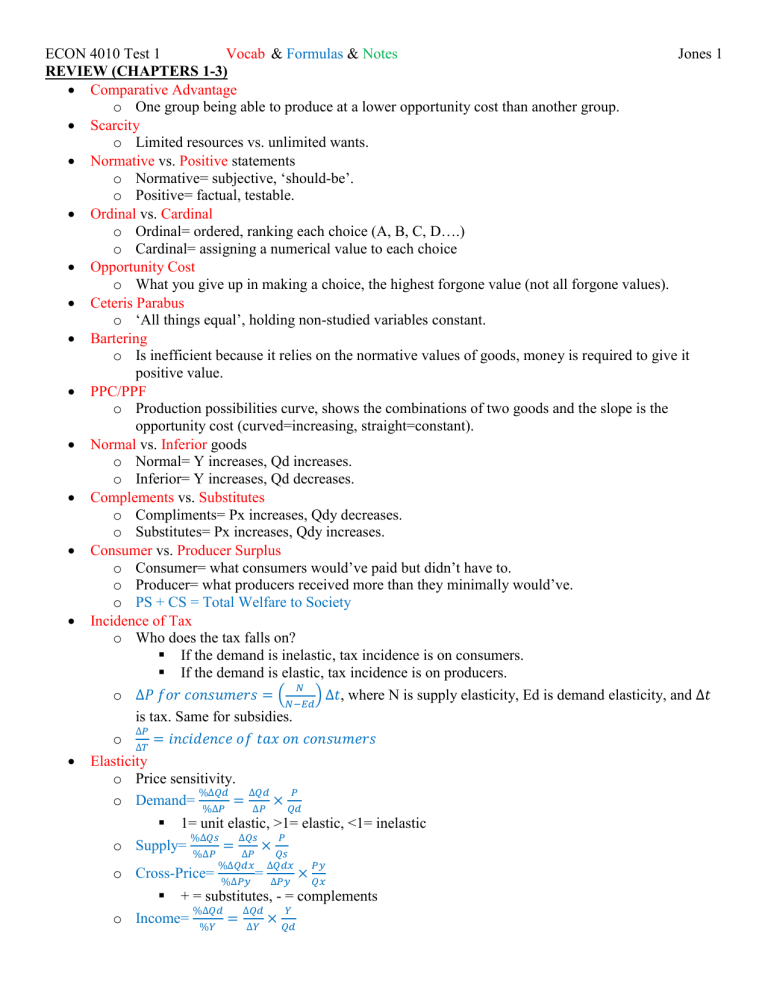
ECON 4010 Test 1
Vocab & Formulas & Notes
Jones 1
REVIEW (CHAPTERS 1-3)
 Comparative Advantage
o One group being able to produce at a lower opportunity cost than another group.
 Scarcity
o Limited resources vs. unlimited wants.
 Normative vs. Positive statements
o Normative= subjective, ‘should-be’.
o Positive= factual, testable.
 Ordinal vs. Cardinal
o Ordinal= ordered, ranking each choice (A, B, C, D….)
o Cardinal= assigning a numerical value to each choice
 Opportunity Cost
o What you give up in making a choice, the highest forgone value (not all forgone values).
 Ceteris Parabus
o ‘All things equal’, holding non-studied variables constant.
 Bartering
o Is inefficient because it relies on the normative values of goods, money is required to give it
positive value.
 PPC/PPF
o Production possibilities curve, shows the combinations of two goods and the slope is the
opportunity cost (curved=increasing, straight=constant).
 Normal vs. Inferior goods
o Normal= Y increases, Qd increases.
o Inferior= Y increases, Qd decreases.
 Complements vs. Substitutes
o Compliments= Px increases, Qdy decreases.
o Substitutes= Px increases, Qdy increases.
 Consumer vs. Producer Surplus
o Consumer= what consumers would’ve paid but didn’t have to.
o Producer= what producers received more than they minimally would’ve.
o PS + CS = Total Welfare to Society
 Incidence of Tax
o Who does the tax falls on?
 If the demand is inelastic, tax incidence is on consumers.
 If the demand is elastic, tax incidence is on producers.
𝑁
o ∆𝑃 𝑓𝑜𝑟 𝑐𝑜𝑛𝑠𝑢𝑚𝑒𝑟𝑠 = (𝑁−𝐸𝑑) ∆𝑡, where N is supply elasticity, Ed is demand elasticity, and ∆𝑡
is tax. Same for subsidies.
∆𝑃
o ∆𝑇 = 𝑖𝑛𝑐𝑖𝑑𝑒𝑛𝑐𝑒 𝑜𝑓 𝑡𝑎𝑥 𝑜𝑛 𝑐𝑜𝑛𝑠𝑢𝑚𝑒𝑟𝑠
 Elasticity
o Price sensitivity.
%∆𝑄𝑑
∆𝑄𝑑
𝑃
o Demand= %∆𝑃 = ∆𝑃 × 𝑄𝑑
 1= unit elastic, >1= elastic, <1= inelastic
%∆𝑄𝑠
∆𝑄𝑠
𝑃
o Supply= %∆𝑃 = ∆𝑃 × 𝑄𝑠
o Cross-Price=
%∆𝑄𝑑𝑥
%∆𝑃𝑦
=
∆𝑄𝑑𝑥
∆𝑃𝑦
𝑃𝑦
× 𝑄𝑥
 + = substitutes, - = complements
%∆𝑄𝑑
∆𝑄𝑑
𝑌
o Income= %𝑌 = ∆𝑌 × 𝑄𝑑
ECON 4010 Test 1
Vocab & Formulas & Notes
Jones 2
 + = normal good, - =inferior good
𝑑𝑄
𝑃𝑥
o Point= × , where the first term is the price for the certain variable, and the second is the
𝑑𝑃
𝑄𝑥
point on the demand curve.
 Price Floor vs. Ceiling
o Floor= above market price, causes a surplus.
o Ceiling= below market price, causes a shortage.
o See graphs.
 Private vs. Public goods
o Private goods= rival (only I can have it) and excludable (you must pay to enjoy the benefits)
o Public good= nonrival and nonexcludable.
o Club good= nonrival and excludable.
 Dead Weight Loss
o The value lost to society because of a tax.
o See graphs.
CHAPTER 4- CONSUMER CHOICE THEORY
 Consumers…...
o Have preferences
o Have constraints
o Consume of bundles of goods
o Maximize utility
 Preferences
o Consumers are…...
 Rational= able to rank preferences
 Maximizing= make the choice that brings most utility
 Difficult to satisfy
 Goods= more is good
 Bads= more is bad
o Modeled by Indifference Curves.
 Assumptions
 Represent utility
 There are lots of them.
 Slopes down and right (diminishing MU)
 They don’t cross.
 Convex/bows inward
 Farther from the origin= more utility.
 Any point on the same indifference curve brings the same amount of utility.
 Indifference Maps show all indifference curves.
 More complimentary goods are U-shaped, more substitutable goods are more of a
constant slope.
𝑀𝑈𝑥1
∆𝑋1
 Slope of indifference curves= 𝑀𝑅𝑆 = − 𝑀𝑈𝑦1 = ∆𝑋2




MU is the derivative of the Utility Function.
Consume X1 until the MU of the last unit of X1 is lower than the utility of the first unit
of X2
𝑀𝑈𝑥1
𝑀𝑈𝑥2
Utility maximizing point at 𝑃1 = 𝑃2
Preferences must have….
 Transitivity
o Consumers prefer x to y and y to z, and therefore x to z (no incomplete
preferences).
ECON 4010 Test 1



Vocab & Formulas & Notes
Jones 3
 Completeness
o Consumers can ordinally rank preferences.
 “More is Better”
Endowment Effect
 People value a good more if they already have it than if they are considering
buying it.
Bounded Rationality
 People have a limited capacity to handle complex problems, so people only pay
attention to taxes when they are high, or their demand is elastic.
Constraints
𝑃1
o Budget constraint slope= 𝑀𝑅𝑇 = − 𝑃2
o Price increases shift an intercept out, price decreases shift an intercept in.
o Credits that can be used for a single good (like gift cards) add a perfectly vertical or horizontal
section on the opposite axis.
o Budget constraint changes change the way people behave.
 Examples:
o Government subsidizes healthcare past a certain point. If the consumer is consuming below this
point, then, if the expenditure increase on healthcare is lower than the subsidy, they will increase
spending to get it.
 See graphs.
o Public School Paradox
 Public schooling is basically an endowment, and education past that is out of pocket and
on the private school budget constraint. To go to private school, you must pay the entire
cost out of pocket, which is higher than the endowment. Or, you can choose public
schools, get a slightly worse education, but be able to spend all that money on AOG. The
second option has a higher utility curve.
 See graphs.
 An individual’s demand curve is derived by:
o 1- changing the price of the good
o 2- drawing new indifference curves and their respective tangent points
o 3- connecting the tangent points in the price consumption curve
o 4- plotting these points on the demand graph
CHAPTER 5- APPLYING CONSUMER CHOICE THEORY
 How does an income change effect the demand curve? Analyzed thru….
o Indifference curves
o Demand curves
o Engel Curve= Income on y-axis, Qd on x-axis
o Income elasticity of demand
o Income changes DO NOT cause substitution.
 How does a price change impact the demand curve?
o Income Effect= Price changes affect your relative purchasing power. If the price of a good goes
down, it’s like your income went up. Seen as quantity difference from the old and new tangent
points.
o Substitution Effect= When prices change, you substitute to the cheaper of two goods. Seen as the
quantity difference between the original tangent point and the point on the original I curve where
the new budget constraint would intersect.
o For normal goods, the effects go the same direction. For inferior goods, they go in the opposite
direction, but the substitution effect is stronger. For Giffen goods (price increases make people
buy more and vice versa, are a huge part of your budget), they work in opposite directions but
the income effect is stronger.
ECON 4010 Test 1
Vocab & Formulas & Notes
Jones 4
o See graphs.
 Labor-Leisure Model
o Happiness is a utility function, the variables being ….
 Consumption= basically working for a wage, which gives you money, which allows you
to consume more the more you work.
 𝐶𝑜𝑛𝑠𝑢𝑚𝑝𝑡𝑖𝑜𝑛 𝐹𝑢𝑛𝑐𝑡𝑖𝑜𝑛 = (𝑊𝑇 + 𝑉) − 𝑊𝐿, where W is wage rate, T is total
time, V is endowment, and L is leisure time.
 Leisure= anything that’s not working. Leisure is a normal good.
o Endowments allow you to consume without working. They raise the budget constraint but DO
NOT affect its slope.
𝑀𝑈𝑙
o Tangent point= 𝑀𝑈𝑐 = 𝑊
𝑀𝑈𝑙

o 𝑀𝑅𝑆 = − 𝑀𝑈𝑐
o Wage Rate= slope of the budget constraint. Increasing wages make it slope steeper downward.
o As wage rises, the income effect wants to increase leisure and the substitution effect wants to
increase work. The substitution effect is stronger until a certain point, then the income is stronger
because of diminishing MUc.
 This makes an individual’s labor supply curve upward sloping at first and then bending
backwards as wage rises.
 This is different than the market labor supply because as wage rises, more people
enter the market for labor when the wage goes past their Reservation Wage. This
wage is higher for people with more vertical indifference curves.
o Examples:
 Government assistance
 All-or-nothing government assistance encourages individuals to not work because
they lose the aid the first hour they work.
 EITC (Earned Income Tax Credit) gives increasing aid for the first hours of work,
then constant aid for the next set of hours, and then diminishing aid for the last
hours. This makes W effectively higher at all hours
 See graphs.
o See graphs.
Save or borrow? An inter-temporal choice.
o Axes are consumption in year 1 (present) and consumption in year 2 (future).
o E is the endowment point. Consumption of C2 past the endowment reflects savings, and
consumption before E on C1 reflects borrowing. Consumption past E on C2 is most realistic.
1
o 𝑀 𝑜𝑓 𝐵𝑢𝑑𝑔𝑒𝑡 𝐶𝑜𝑛𝑠𝑡𝑟𝑎𝑖𝑛𝑡 = 𝐼𝑛𝑡𝑒𝑟𝑒𝑠𝑡 𝑅𝑎𝑡𝑒 = 1+𝑟
 Interest rate changes will always rotate the budget constraint through E.
 Rising interest rate= You can’t consume as much in the present because the price of
borrowing rose, but you can consume more in the future because your savings are
increasing.
o Expecting a loss or gain of future income shifts the whole constraint, not just for one period. This
is because of Consumption Smoothing, consuming similar amounts in each period after factoring
in changes.
o Personal Discount Rate= How much money is worth to you now vs. in the future.
o Substitution effect makes you consume more in the future because the intercept is shifting out.
Income effect makes you consume more in the present (this is because if you spend more now
and save less, the savings value will be closer to the original savings because of the higher
interest rate. Whichever one is stronger comes down to preferences, but regardless you consume
more in the future.
o See graphs.
ECON 4010 Test 1
Vocab & Formulas & Notes
Jones 5
 Insurance
o Most people are Risk Averse, meaning their total utility rises at a diminishing rate with increased
risk/income.
o Buying insurance will decrease income and hence TU but guarantees that this is the lowest TU
can go. Without insurance, TU has the potential to be extremely low in the event of a disaster,
but if there is no disaster, TU is at its highest because you keep all the income.
o See graphs.