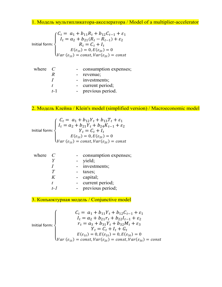
1. Модель мультипликатора-акселератора / Model of a multiplier-accelerator
𝐶𝑡 = 𝑎1 + 𝑏11 𝑅𝑡 + 𝑏12 𝐶𝑡−1 + 𝜀1
𝐼𝑡 = 𝑎2 + 𝑏21 (𝑅𝑡 − 𝑅𝑡−1 ) + 𝜀2
Initial form:
𝑅𝑡 = 𝐶𝑡 + 𝐼𝑡
𝐸(𝜀1𝑡 ) = 0, 𝐸(𝜀2𝑡 ) = 0
{𝑉𝑎𝑟 (𝜀1𝑡 ) = 𝑐𝑜𝑛𝑠𝑡, 𝑉𝑎𝑟(𝜀2𝑡 ) = 𝑐𝑜𝑛𝑠𝑡
where C
R
I
t
t-1
-
consumption expenses;
revenue;
investments;
current period;
previous period.
2. Модель Клейна / Klein's model (simplified version) / Macroeconomic model
𝐶𝑡 = 𝑎1 + 𝑏12 𝑌𝑡 + 𝑏13 𝑇𝑡 + 𝜀1
𝐼𝑡 = 𝑎2 + 𝑏21 𝑌𝑡 + 𝑏24 𝐾𝑡−1 + 𝜀2
𝑌𝑡 = 𝐶𝑡 + 𝐼𝑡
Initial form:
𝐸(𝜀1𝑡 ) = 0, 𝐸(𝜀2𝑡 ) = 0
{𝑉𝑎𝑟 (𝜀1𝑡 ) = 𝑐𝑜𝑛𝑠𝑡, 𝑉𝑎𝑟(𝜀2𝑡 ) = 𝑐𝑜𝑛𝑠𝑡
where C
Y
I
T
K
t
t-1
-
consumption expenses;
yield;
investments;
taxes;
capital;
current period;
previous period;
3. Конъюктурная модель / Conjunctive model
Initial form:
𝐶𝑡 = 𝑎1 + 𝑏11 𝑌𝑡 + 𝑏12 𝐶𝑡−1 + 𝜀1
𝐼𝑡 = 𝑎2 + 𝑏21 𝑟𝑡 + 𝑏22 𝐼𝑡−1 + 𝜀2
𝑟𝑡 = 𝑎3 + 𝑏31 𝑌𝑡 + 𝑏32 𝑀𝑡 + 𝜀3
𝑌𝑡 = 𝐶𝑡 + 𝐼𝑡 + 𝐺𝑡
𝐸(𝜀1𝑡 ) = 0, 𝐸(𝜀2𝑡 ) = 0, 𝐸(𝜀3𝑡 ) = 0
{𝑉𝑎𝑟 (𝜀1𝑡 ) = 𝑐𝑜𝑛𝑠𝑡, 𝑉𝑎𝑟(𝜀2𝑡 ) = 𝑐𝑜𝑛𝑠𝑡, 𝑉𝑎𝑟(𝜀3𝑡 ) = 𝑐𝑜𝑛𝑠𝑡
where C
Y
I
r
M
G
t
t-1
-
consumption expenses;
GDP;
investments;
interest rate;
money supply;
government expenses;
current period;
previous period.
4. IS-LM model
𝐶𝑡 = 𝑎0 + 𝑎1 ∙ (𝑌𝑡 − 𝑇𝑡 ) + 𝜀1𝑡
𝐼𝑡 = 𝑏0 + 𝑏1 ∙ 𝑅𝑡 + 𝜀2𝑡
𝐿𝑡 = 𝑐0 +𝑐1 ∙ 𝑅𝑡 + 𝑌𝑡 + 𝜀3𝑡
𝑌𝑡 = 𝐶𝑡 + 𝐼𝑡 + 𝐺𝑡
Initial form:
𝐿𝑡 = 𝑀𝑡
𝐸(𝜀1𝑡 ) = 0, 𝐸(𝜀2𝑡 ) = 0, 𝐸(𝜀3𝑡 ) = 0
{𝑉𝑎𝑟 (𝜀1𝑡 ) = 𝑐𝑜𝑛𝑠𝑡, 𝑉𝑎𝑟(𝜀2𝑡 ) = 𝑐𝑜𝑛𝑠𝑡, 𝑉𝑎𝑟(𝜀3𝑡 ) = 𝑐
5. The Samuelson-Hicks econometric Model
𝐶𝑡 = 𝑎0 + 𝑎1 ∙ 𝑌𝑡−1 + 𝜀1𝑡
𝐼𝑡 = 𝑏0 + 𝑏1 ∙ (𝑌𝑡−1 − 𝑌𝑡−2 ) + 𝜀2𝑡
𝐺𝑡 = 𝑔1 ∙ 𝐺𝑡−1 + 𝜀3𝑡
Initial form:
𝑌𝑡 = 𝐶𝑡 + 𝐼𝑡 + 𝐺𝑡
𝐸(𝜀1𝑡 ) = 0, 𝐸(𝜀2𝑡 ) = 0, 𝐸(𝜀3𝑡 ) = 0
{𝑉𝑎𝑟 (𝜀1𝑡 ) = 𝑐𝑜𝑛𝑠𝑡, 𝑉𝑎𝑟(𝜀2𝑡 ) = 𝑐𝑜𝑛𝑠𝑡, 𝑉𝑎𝑟(𝜀3𝑡 ) = 𝑐
6. Keynes's models for open and closed economies with and without government intervention
The Keynesian econometric model of a closed economy without government intervention
𝐶𝑡 = 𝑎0 + 𝑎1 𝑌𝑡 + 𝑎2 𝑌𝑡−1 + ℇ1𝑡
𝐼𝑡 = 𝑏0 + 𝑏1 𝑌𝑡 + 𝑏2 𝑌𝑡−1 + ℇ2𝑡
𝑌𝑡 = 𝐶𝑡 + 𝐼𝑡 + 𝐺𝑡
Initial form:
𝐸 (𝜀1𝑡 ) = 0, 𝐸 (𝜀2𝑡 ) = 0
{𝑉𝑎𝑟 (𝜀1𝑡 ) = 𝑐𝑜𝑛𝑠𝑡, 𝑉𝑎𝑟(𝜀2𝑡 ) = 𝑐𝑜𝑛𝑠𝑡
𝐶𝑡 = 𝛼0 + 𝛼1 𝑌𝑡−1 + 𝛼2 𝐺𝑡 + 𝜇0
Reduced form: { 𝐼𝑡 = 𝛽0 + 𝛽1 𝑌𝑡−1 + 𝛽2 𝐺𝑡 + 𝜇1
𝑌𝑡 = 𝛾0 + 𝛾1 𝑌𝑡−1 + 𝛾2 𝐺𝑡 + 𝜇2
The Keynesian econometric model of closed economy with government intervention
𝐶𝑡 = 𝑎0 + 𝑎1 (𝑌𝑡 − 𝑇𝑡 ) + ℇ1𝑡
𝐼𝑡 = 𝑏0 + 𝑏1 𝑌𝑡 + 𝑏2 𝑅𝑡 + ℇ2𝑡
𝑌𝑡 = 𝐶𝑡 + 𝐼𝑡 + 𝐺𝑡
Initial form:
𝐸(𝜀1𝑡 ) = 0, 𝐸(𝜀2𝑡 ) = 0
{𝑉𝑎𝑟 (𝜀1𝑡 ) = 𝑐𝑜𝑛𝑠𝑡, 𝑉𝑎𝑟(𝜀2𝑡 ) = 𝑐𝑜𝑛𝑠𝑡
𝐶𝑡 = 𝛼0 + 𝛼1 𝑇𝑡 + 𝛼2 𝑅𝑡 + 𝛼3 𝐺𝑡 + 𝜇0
Reduced form:{ 𝐼𝑡 = 𝛽0 + 𝛽1 𝑇𝑡 + 𝛽2 𝑅𝑡 + 𝛽3 𝐺𝑡 + 𝜇1
𝑌𝑡 = 𝛾0 + 𝛾1 𝑇𝑡 + 𝛾2 𝑅𝑡 + 𝛾3 𝐺𝑡 + 𝜇2
The Keynesian econometric model of open economy
𝐶𝑡 = 𝑎0 + 𝑎1 𝑌𝑡 + 𝑎2 𝐶𝑡−1 + 𝜀1𝑡
𝐼𝑡 = 𝑏0 + 𝑏1 𝑌𝑡 + 𝑏2 𝑟𝑡 + 𝜀2𝑡
𝑟𝑡 = 𝑐0 + 𝑐1 𝑌𝑡 + 𝑐2 𝑀𝑡 + 𝑐3 𝑟𝑡−1 + 𝜀3𝑡
Initial form:
𝑌𝑡 = 𝐶𝑡 + 𝐼𝑡 + 𝐺𝑡
𝐸(𝜀1𝑡 ) = 0, 𝐸(𝜀2𝑡 ) = 0, 𝐸(𝜀3𝑡 ) = 0
{𝑉𝑎𝑟 (𝜀1𝑡 ) = 𝑐𝑜𝑛𝑠𝑡, 𝑉𝑎𝑟(𝜀2𝑡 ) = 𝑐𝑜𝑛𝑠𝑡, 𝑉𝑎𝑟(𝜀3𝑡 ) = 𝑐𝑜𝑛𝑠𝑡
𝐶𝑡 = 𝛼0 + 𝛼1 𝐶𝑡−1 + 𝛼2 𝑀𝑡 + 𝛼3 𝑟𝑡−1 + 𝛼4 𝐺𝑡 + 𝜇0
𝐼 = 𝛽0 + 𝛽1 𝐶𝑡−1 + 𝛽2 𝑀𝑡 + 𝛽3 𝑟𝑡−1 + 𝛽4 𝐺𝑡 + 𝜇1
Reduced form: { 𝑡
𝑟𝑡 = 𝛾0 + 𝛾1 𝐶𝑡−1 + 𝛾2 𝑀𝑡 + 𝛾3 𝑟𝑡−1 + 𝛾4 𝐺𝑡 + 𝜇2
𝑌𝑡 = 𝛿0 + 𝛿1 𝐶𝑡−1 + 𝛿2 𝑀𝑡 + 𝛿3 𝑟𝑡−1 + 𝛿4 𝐺𝑡 + 𝜇3
Mt – денежная масса
7. Модель денежного рынка / Money market model
Initial form:
𝑅𝑡 = 𝑎1 + 𝑏11 𝑀𝑡 + 𝑏12 𝑌𝑡 + 𝜀1
𝑌𝑡 = 𝑎2 + 𝑏21 𝑅𝑡 + 𝑏22 𝐼𝑡 + 𝜀2
𝐸(𝜀1𝑡 ) = 0, 𝐸(𝜀2𝑡 ) = 0
{𝑉𝑎𝑟 (𝜀1𝑡 ) = 𝑐𝑜𝑛𝑠𝑡, 𝑉𝑎𝑟(𝜀2𝑡 ) = 𝑐𝑜𝑛𝑠𝑡
where R
Y
I
M
t
-
Interest rate;
GDP;
investments;
money supply;
current period;
8. Модель Менгеса / Menges model
𝑌𝑡 = 𝑎1 + 𝑏11 𝑌𝑡−1 + 𝑏12 𝐼𝑡 + 𝜀1
𝐼𝑡 = 𝑎2 + 𝑏21 𝑌𝑡 + 𝑏22 𝑄𝑡 + 𝜀2
𝐶𝑡 = 𝑎3 + 𝑏31 𝑌 + 𝑏32 С𝑡−1 + 𝑏33 𝑃𝑡 + 𝜀3
𝑄𝑡 = 𝑎4 + 𝑏41 𝑄𝑡−1 + 𝑏42 𝑅𝑡 + 𝜀4
Initial form:
𝐸(𝜀1𝑡 ) = 0, 𝐸(𝜀2𝑡 ) = 0, 𝐸(𝜀3𝑡 ) = 0, 𝐸(𝜀4𝑡 ) = 0
{𝑉𝑎𝑟 (𝜀1𝑡 ) = 𝑐𝑜𝑛𝑠𝑡, 𝑉𝑎𝑟(𝜀2𝑡 ) = 𝑐𝑜𝑛𝑠𝑡, 𝑉𝑎𝑟 (𝜀3𝑡 ) = 𝑐𝑜𝑛𝑠𝑡, 𝑉𝑎𝑟(𝜀4𝑡 ) = 𝑐𝑜𝑛𝑠𝑡
where C
Y
I
Q
P
R
t
t-1
-
consumption expenses;
GDP;
investments;
gross profit of the economy;
cost of living index;
industrial output;
current period;
previous period.
9. Модели финансовых рынков / Models of financial markets
𝑅𝑡 = 𝑎1 + 𝑏12 𝑌𝑡 + 𝑏14 𝑀𝑡 + 𝜀1
𝑌𝑡 = 𝑎2 + 𝑏21 𝑅𝑡 + 𝑏23 𝐼𝑡 + 𝑏25 𝐺𝑡 + 𝜀2
𝐼𝑡 = 𝑎3 + 𝑏31 𝑅𝑡 + 𝜀3
𝑌𝑡 = 𝐶𝑡 + 𝐼𝑡 + 𝐺𝑡
Initial form:
𝐸(𝜀1𝑡 ) = 0, 𝐸(𝜀2𝑡 ) = 0, 𝐸(𝜀3𝑡 ) = 0
{𝑉𝑎𝑟 (𝜀1𝑡 ) = 𝑐𝑜𝑛𝑠𝑡, 𝑉𝑎𝑟(𝜀2𝑡 ) = 𝑐𝑜𝑛𝑠𝑡, 𝑉𝑎𝑟(𝜀3𝑡 ) = 𝑐𝑜𝑛𝑠𝑡
where
R
-
Interest rate;
Y
-
GDP;
I
-
investments;
M
-
money supply;
G
-
government expenses;
t
-
current period;
10.Макроэконометрические модели на примере реальных экономик /
Macroeconometric models on the example of real economies
(США)
𝐶𝑡 = 𝑎1 + 𝑏11 𝑌𝑡 + 𝑏12 𝐶𝑡−1 + 𝜀1𝑡
𝐼𝑡 = 𝑎2 + 𝑏21 𝑌𝑡 + 𝑏23 𝑟𝑡 + 𝜀2𝑡
𝑟𝑡 = 𝑎3 + 𝑏31 𝑌𝑡 + 𝑏34 𝑀𝑡 + 𝑏35 𝑟𝑡−1 + 𝜀3𝑡
Initial form:
𝑌𝑡 = 𝐶𝑡 + 𝐼𝑡 + 𝐺𝑡
𝐸(𝜀1𝑡 ) = 0, 𝐸(𝜀2𝑡 ) = 0, 𝐸(𝜀3𝑡 ) = 0
{𝑉𝑎𝑟 (𝜀1𝑡 ) = 𝑐𝑜𝑛𝑠𝑡, 𝑉𝑎𝑟(𝜀2𝑡 ) = 𝑐𝑜𝑛𝑠𝑡, 𝑉𝑎𝑟(𝜀3𝑡 ) = 𝑐𝑜𝑛𝑠𝑡
where C
Y
I
r
M
G
t
t-1
-
consumption expenses;
GDP;
investments;
interest rate;
money supply;
government expenses;
current period;
previous period.
11. Model specifications: structural, reduced, evaluated
1st example
Structural:
Reduced:
2nd example from classwork
Examples from her textbook(as in our HW):
Structural:
Estimated:
12. Taking into account the principles of the specification when developing the
structural form of the model
13. Types of variables: exogenous, endogenous, current, lagged. Features of their
inclusion in the model.
The economic variables involved in any econometric model fall into four types:
1) exogenous (independent) - variables whose values are set from the outside. To a
certain extent, these variables are controllable (x);
2) endogenous (dependent) - variables, the values of which are determined within the
model, or interdependent (y);
3) lagged - exogenous or endogenous variables in the econometric model, related to
previous points in time and are in the equation with variables related to the current
point in time;
4) predefined (explanatory variables) -lag (xi − 1) and current (x) exogenous
variables, as well as lagged endogenous variables (yi - 1).
Any econometric model is designed to explain the values of one or more current
endogenous variables depending on the values of predefined variables.
14. Methods for preparing data for modeling. Dimensional accounting, scaling,
interpolation, extrapolation
Interpolation
We could use our function to predict the value of the dependent variable for an
independent variable that is in the midst of our data. In this case, we are performing
interpolation. Suppose that data with x between 0 and 10 is used to produce a
regression line y = 2x+ 5. We can use this line of best fit to estimate the y value
corresponding to x = 6. Simply plug this value into our equation and we see that y =
2(6) + 5 =17. Because our x value is among the range of values used to make the line
of best fit, this is an example of interpolation.
Extrapolation
We could use our function to predict the value of the dependent variable for an
independent variable that is outside the range of our data. In this case, we are
performing extrapolation.
Suppose as before that data with x between 0 and 10 is used to produce a regression
line y = 2x + 5. We can use this line of best fit to estimate the y value corresponding
to x = 20. Simply plug this value into our equation
and we see that y = 2(20) + 5 =45. Because our x value is not among the range of
values used to make the line of best fit, this is an example of extrapolation.
Caution
Of the two methods, interpolation is preferred. This is because we have a greater
likelihood of obtaining a valid estimate. When we use extrapolation, we are making
the assumption that our observed trend continues for values of x outside the range we
used to form our model. This may not be the case, and so we must be very careful
when using extrapolation techniques.
15. Construction of a matrix of pairwise correlations. Identification of the type of
correlation, analysis of possible multicollinearity in the regression model.
Multicollinearity occurs when independent variables in a regression model
are correlated. This correlation is a problem because independent variables should
be independent. If the degree of correlation between variables is high enough, it
can cause problems when you fit the model and interpret the results.
A key goal of regression analysis is to isolate the relationship between each
independent variable and the dependent variable. The interpretation of a regression
coefficient is that it represents the mean change in the dependent variable for each
1 unit change in an independent variable when you hold all of the other
independent variables constant. That last portion is crucial for our discussion about
multicollinearity.
The idea is that you can change the value of one independent variable and
not the others. However, when independent variables are correlated, it indicates
that changes in one variable are associated with shifts in another variable. The
stronger the correlation, the more difficult it is to change one variable without
changing another. It becomes difficult for the model to estimate the relationship
between each independent variable and the dependent variable independently
because the independent variables tend to change in unison.
There are two basic kinds of multicollinearity:
Structural multicollinearity: This type occurs when we create a model term
using other terms. In other words, it’s a byproduct of the model that we specify
rather than being present in the data itself. For example, if you square term X to
model curvature, clearly there is a correlation between X and X2.
Data multicollinearity: This type of multicollinearity is present in the data
itself rather than being an artifact of our model. Observational experiments are
more likely to exhibit this kind of multicollinearity.
Correlation is a statistical measure that indicates the extent to which two or
more variables move together. A positive correlation indicates that the variables
increase or decrease together. A negative correlation indicates that if one variable
increases, the other decreases, and vice versa.
The correlation coefficient indicates the strength of the linear relationship
that might be existing between two variables.
The correlation matrix below for the numeric features indicates a high
correlation of 0.82 and 0.65 between (TotalCharges, contract_age) and
(TotalCharges, MonthlyCharges) respectively. This indicates a possible problem of
multicollinearity and the need for further investigation.
16. Construction of scatter diagrams. Analysis of residuals to identify
autocorrelation and heteroscedasticity.
According to this assumption there is linear relationship between the
features and target. Linear regression captures only linear relationship. This can be
validated by plotting a scatter plot between the features and the target.
The first scatter plot of the feature TV vs Sales tells us that as the money
invested on Tv advertisement increases the sales also increases linearly and the
second scatter plot which is the feature Radio vs Sales also shows a partial linear
relationship between them, although not completely linear.
Autocorrelation occurs when the residual errors are dependent on each
other. The presence of correlation in error terms drastically reduces model’s
accuracy. This usually occurs in time series models where the next instant is
dependent on previous instant.
Autocorrelation can be tested with the help of Durbin-Watson test. The null
hypothesis of the test is that there is no serial correlation. The Durbin-Watson test
statistics is defined as:
The test statistic is approximately equal to 2*(1-r) where r is the sample
autocorrelation of the residuals. Thus, for r == 0, indicating no serial correlation,
the test statistic equals 2. This statistic will always be between 0 and 4. The closer
to 0 the statistic, the more evidence for positive serial correlation. The closer to 4,
the more evidence for negative serial correlation.
Suppose the regression model we want to test for heteroskedasticity is the
one in Equation:
yi=β1+β2xi2+...+βKxiK+ei
The test we are construction assumes that the variance of the errors is a
function h of a number of regressors zs, which may or may not be present in the
initial regression model that we want to test. Equation shows the general form of
the variance function.
var(yi)=E(e2i)=h(α1+α2zi2+...+αSziS)
The variance var(yi) is constant only if all the coefficients of the regressors z
in Equation are zero, which provides the null hypothesis of our heteroskedasticity
test shown in Equation:
H0:α2=α3=...αS=0
Since the presence of heteroskedasticity makes the lest-squares standard
errors incorrect, there is a need for another method to calculate them. White robust
standard errors are such a method.
The R function that does this job is hccm (), which is part of the car package
and yields a heteroskedasticity-robust coefficient covariance matrix. This matrix
can then be used with other functions, such as coeftest () (instead of summary),
waldtest () (instead of anova), or linear Hypothesis () to perform hypothesis
testing. The function hccm() takes several arguments, among which is the model
for which we want the robust standard errors and the type of standard errors we
wish to calculate. type can be “constant” (the regular homoscedastic errors), “hc0”,
“hc1”, “hc2”, “hc3”, or “hc4”; “hc1” is the default type in some statistical software
packages.
17. Gauss-Markov theorem. Features of its recording in the structural and reduced
forms of the model.
Christopher Dougherty Introduction to Econometry Страница 83-84 пункт 3.6 Текст
взят из: https://goo.su/3V9Q
The Gauss-Markov theorem states that if your linear regression model satisfies
classical assumptions, then ordinary least squares (OLS) regression produces
unbiased estimates that have the smallest variance of all possible linear estimators.
The Gauss-Markov theorem famously states that OLS is BLUE. BLUE is an
acronym for the Best Linear Unbiased Estimator
In this context, the definition of “best” refers to the minimum variance or the
narrowest sampling distribution. More specifically, when your model satisfies the
assumptions, OLS coefficient estimates follow the tightest possible sampling
distribution of unbiased estimates compared to other linear estimation methods.
Gauss–Markov Condition 1: E(ui ) = 0 for All Observations
The first condition is that the expected value of the disturbance term in any
observation should be 0. Sometimes it will be positive, sometimes negative, but it
should not have a systematic tendency in either direction.
Gauss–Markov Condition 2: Population Variance of ui Constant for All
Observations
Gauss–Markov Condition 3: Observations of the error term are uncorrelated with
each other (no autocorrelation)
One observation of the error term should not predict the next observation. For
instance, if the error for one observation is positive and that systematically
increases the probability that the following error is positive, that is a positive
correlation. If the subsequent error is more likely to have the opposite sign, that is a
negative correlation. This problem is known both as serial correlation and
autocorrelation.
Gauss–Markov Condition 4: All independent variables are uncorrelated with the
error term
Gauss–Markov Condition 5: The error term has a constant variance (no
heteroscedasticity)
18. Violation of the premises of the Gauss-Markov theorem and possible ways
to eliminate them
How to fix autocorrelation:
How to fix heteroscedasticity:
21. Confidence intervals when checking the adequacy of the model
Any hypothetical value of β2 that satisfies (3.58) will therefore automatically be
compatible with the estimate b2, that is, will not be rejected by it. The set of all such
values, given by the interval between the lower and upper limits of the inequality, is
known as the confidence interval for β2.
Note that the center of the confidence interval is b2 itself. The limits are equidistant on
either side. Note also that, since the value of tcrit depends upon the choice of significance
level, the limits will also depend on this choice. If the 5 percent significance level is
adopted, the corresponding confidence interval is known as the 95 percent confidence
interval. If the 1 percent level is chosen, one obtains the 99 percent confidence interval,
and so on.
If the Yp values from the control sample are covered by a confidence interval — the
model is considered adequate, otherwise it is subject to revision.
22. Tests for the significance of the model coefficients.
23. Model specification quality test
𝑅2
𝑛−𝑚−1
𝐹=
∙
2
1−𝑅
𝑚
F-test estimation quality of the regression equation - is to test the hypothesis
H0 about the statistical insignificance of regression equations and the index of
correlation. If F is critical < F is actual, then the H0 hypothesis about the random
nature of the estimated characteristics is rejected and their statistical significance
and reliability are recognized. If F is critical > F is actual, then the H0 hypothesis is
not rejected and the statistical insignificance and unreliability of the regression
equation is recognized.
24. R2 test
The coefficient of determination is the proportion of the variance of the dependent
variable that is explained by the dependency model under consideration, that is, by
the explanatory variables.
∑(𝑦 − 𝑦̂)2
𝑆𝑆𝑒
𝑅 =1−
=
1
−
∑(𝑦 − 𝑦̅)2
𝑆𝑆общ
2
The coefficient varies in the range from zero to one. The higher the coefficient, the
higher the quality of the approximation. The complication, increase of its
parameters, at constant scope of observations leads to the increase of correlation
R2 and R. To account for this feature, the adjusted coefficient of determination is
calculated.
2
𝑅𝑎𝑑𝑗𝑢𝑠𝑡𝑒𝑑
= 1 − (1 − 𝑅2 ) ∙
𝑛−1
𝑛−𝑚−1
The adjusted coefficient of determination is used to estimate the actual tightness of
the relationship between the result and the factors and to compare models with a
different number of parameters. In the first case, pay attention to the proximity of
the adjusted and uncorrected coefficient of determination. If these indicators are
close to one and differ slightly, then the model is considered good.
25. Relationship between R2 and F test
In general, F-test is any statistical test in which the test statistic has an F-distribution
under the null hypothesis. It is most often used in comparison of models that have
been fitted to a data set with an intention to find the model that better fits the
population from which the data were sampled.
Such F-tests mainly arise when the models have been fitted to the data using least
squares.
The determination index R2 is used to test the overall significance of the nonlinear
regression equation by Fisher's F-test:
𝐹=
𝑅2
𝑛−𝑚−1
∙
1 − 𝑅2
𝑚
Where R2 is the index of determination.
n is the number of observations;
m is the number of parameters for variables x.
Having calculated F from our value of R2, we look up Fcrit, the critical level of F, in
the appropriate table. If F is greater than Fcrit, we reject the null hypothesis and
conclude that the "explanation" of Y is better than is likely to have arisen by chance,
R2 is non-random and quality of specification is high.
F-test is used to assess the quality of R2.
26. Properties of estimates of the coefficients of the linear regression model
Usually, much attention is given to the following properties of estimators:
unbiasedness, consistency, and efficiency.
Unbiasedness is a property of a statistical estimate, the mathematical expectation of
which is equal to the true value of the parameter being estimated. The bias of the
estimate means the presence of systematic errors in the estimate, i.e., the biased
estimate overestimates or underestimates the true value of the parameter.
Efficiency is a property of a statistical estimate that, for a given sample size N, has the
smallest possible variance, i.e., the possible values of the effective estimate on
average lie closer to its mean value (if the estimate is also unbiased, then, therefore, to
the true value of the estimated parameter ) than the possible values of other estimates.
Thus, an effective unbiased estimate provides the best estimate accuracy.
The estimate of the coefficient is called consistent if, with an increase in the sample
size, the values of the estimate tend in probability to the true value of the parameter
being estimated.