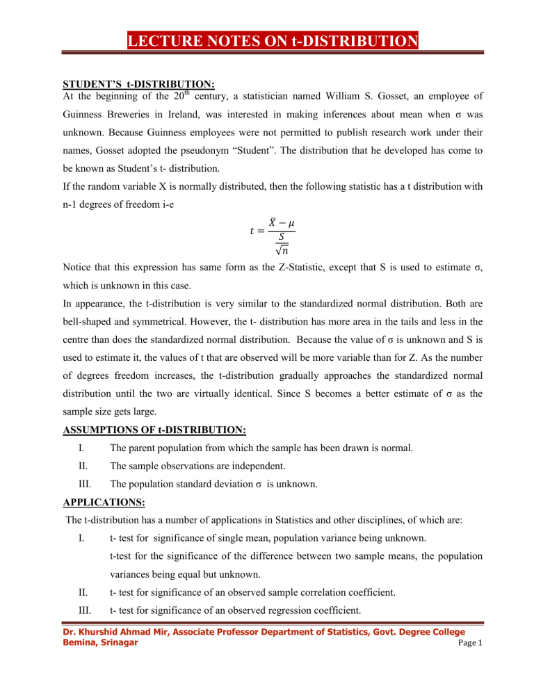
LECTURE NOTES ON t-DISTRIBUTION
STUDENT’S t-DISTRIBUTION:
At the beginning of the 20th century, a statistician named William S. Gosset, an employee of
Guinness Breweries in Ireland, was interested in making inferences about mean when σ was
unknown. Because Guinness employees were not permitted to publish research work under their
names, Gosset adopted the pseudonym “Student”. The distribution that he developed has come to
be known as Student’s t- distribution.
If the random variable X is normally distributed, then the following statistic has a t distribution with
n-1 degrees of freedom i-e
𝑡=
𝑋−𝜇
𝑆
𝑛
Notice that this expression has same form as the Z-Statistic, except that S is used to estimate σ,
which is unknown in this case.
In appearance, the t-distribution is very similar to the standardized normal distribution. Both are
bell-shaped and symmetrical. However, the t- distribution has more area in the tails and less in the
centre than does the standardized normal distribution. Because the value of σ is unknown and S is
used to estimate it, the values of t that are observed will be more variable than for Z. As the number
of degrees freedom increases, the t-distribution gradually approaches the standardized normal
distribution until the two are virtually identical. Since S becomes a better estimate of σ as the
sample size gets large.
ASSUMPTIONS OF t-DISTRIBUTION:
I.
The parent population from which the sample has been drawn is normal.
II.
The sample observations are independent.
III.
The population standard deviation σ is unknown.
APPLICATIONS:
The t-distribution has a number of applications in Statistics and other disciplines, of which are:
I.
t- test for significance of single mean, population variance being unknown.
t-test for the significance of the difference between two sample means, the population
variances being equal but unknown.
II.
t- test for significance of an observed sample correlation coefficient.
III.
t- test for significance of an observed regression coefficient.
Dr. Khurshid Ahmad Mir, Associate Professor Department of Statistics, Govt. Degree College
Bemina, Srinagar
Page 1
LECTURE NOTES ON t-DISTRIBUTION
TEST FOR SINGLE MEAN:
Suppose we are interested to test:
a). If the given normal population has a specified value of the population mean say 𝜇0 .
b). If the sample mean 𝑥 differs significantly from specified value of population mean.
c). If a given random sample x1, x2,…………xn of size n has been drawn from a normal population
with specified mean 𝜇0 .
Basically, all the three problems are same. For all the cases we set up the null hypothesis as:
𝐻0 = 𝜇 = 𝜇0 i.e the population mean is 𝜇.
Under H0, the test statistic is
𝑡=
1
Where 𝑆 2 = 𝑛−1
𝑋 − 𝜇0
~𝑡𝑛 −1
𝑆
𝑛
𝑥𝑖 − 𝑥 2 . The above test statistic is computed and is compared with the
tabulated value of t for (n-1) d.f at certain level of significance. If the calculated value of t is lea
than
the
tabulated
value
of
t,
then
H0
is
accepted,
otherwise
rejected.
Ex: The life expectancy of people in the year 1970 in Brazil is expected to be 50 years. A survey
was conducted in eleven regions of Brazil and the data obtained are given below. Do the data
confirm the expected view.
Life expectancy (Years)x: 54.2, 50.4, 44.2, 49.7, 55.4, 57.0, 58.2, 56.6, 61.9, 57.5, 53.4
Sol: Here we have to test, H0=𝜇 = 50 against H1≠ 50
Under H0, the test statistic t is
𝑋 − 𝜇0
𝑡=
~𝑡𝑛 −1
𝑆
𝑛
Here 𝑥 =
598.5
11
1
= 54.41 and 𝑠 2 = 𝑛 −1
𝑥𝑖 − 𝑥 2 =
1
𝑛−1
𝑥𝑖 2 −
𝑥𝑖 2
𝑛
1
=10 32799.91 − 598.5
2
11
= 23.607
Therefore s= 4.859
Therefore t= 14.626/40859= 3.01.
Dr. Khurshid Ahmad Mir, Associate Professor Department of Statistics, Govt. Degree College
Bemina, Srinagar
Page 2
LECTURE NOTES ON t-DISTRIBUTION
The tabulated value of t at α = 0.05 and 10 d.f is 2.228. Since calculated t is greater than the
tabulated value of t. Therefore, H0 is rejected and we conclude that the life expectancy is more than
5o years.
t- TEST FOR DIFFERENCE OF MEANS
Suppose we want to test if two independent samples have been drawn from two normal populations
having the same means, the population variances being equal.
Let x1, x2,…………xn1 and y1, y2,…………yn2 be two independent random samples from the given
normal populations. We set up the null hypothesis H0: 𝜇𝑥 = 𝜇𝑦 i.e the two samples have been
drawn from the normal populations with the same means. In other words, the sample means 𝑥 and
𝑦 do not differ significantly. Under the assumption that 𝜎1 2 = 𝜎2 2 = 𝜎 2 i.e population variances are
equal but unknown. The test statistic under H0 is
𝑡=
Where 𝑆 2 = 𝑛
1
1 +𝑛 2 −2
𝑥𝑖 − 𝑥
2
+
𝑥−𝑦
~𝑡𝑛 1 +𝑛 2 −2
1
1
𝑆 𝑛 +𝑛
1
2
𝑦𝑖 − 𝑦
2
Proof: Here we know that
𝑍=
𝑥−𝑦 −𝐸 𝑥−𝑦
𝑉( 𝑥 − 𝑦
~𝑁(0,1)
But 𝐸 𝑥 − 𝑦 = 𝐸(𝑥 ) - 𝐸 𝑦 = 𝜇𝑥 − 𝜇𝑦 =0 (By assumption)
and 𝑉( 𝑥 − 𝑦 =𝑉(𝑥)+ V(𝑦 )=
𝜎1 2
𝑛1
+
𝜎2 2
𝑛1
= 𝜎2
1
𝑛1
1
+𝑛
2
(By assumption)
Therefore
𝑥−𝑦
𝑍=
𝜎2
1
1
𝑛1 + 𝑛2
~𝑁(0,1)
Let
2
𝜒 =
𝑥𝑖 − 𝑥
2
+
𝜎2
𝑦𝑖 − 𝑦
2
Then Fisher’s t- statistic is given by
Dr. Khurshid Ahmad Mir, Associate Professor Department of Statistics, Govt. Degree College
Bemina, Srinagar
Page 3
LECTURE NOTES ON t-DISTRIBUTION
𝑡=
𝑍
𝜒2
𝑛1 + 𝑛2 − 2
Which gives
𝑡=
𝑥−𝑦
1
1
𝑆 𝑛 +𝑛
1
2
~𝑡𝑛 1 +𝑛 2 −2
Now by comparing the computed value of t with the tabulated value of t for 𝑛1 + 𝑛2 − 2 d.f at a
certain level of significance, we may reject or accept the null hypothesis.
In case if the assumption 𝜎1 2 = 𝜎2 2 = 𝜎 2 does not hold , then the t- statistic is given as:
𝑡=
𝑥−𝑦
𝑠1 2 𝑠2 2
𝑛1 + 𝑛2
PAIRED t- TEST FOR DIFFERENCE OF MEANS:
In the t-test for difference of means, the two samples were independent of each other. Let us now
take a particular situation where
i)
The sample sizes are equal i.e n1 and n2=n
ii)
The sample observations x1, x2,…………xn1 and y1, y2,…………yn2 are nor completely
independent but are dependent in pairs i.e (x1,y1),(x2,y2)……..(xn,yn) corresponding to
ist, 2nd …….nth unit respectively.
Let di=xi-yi (i= 1,2 ….n) denote the difference in the observations for ith unit.
Under the null hypothesis that the increments are just by chance i.e H0: 𝜇𝑥 = 𝜇𝑦 , the test
statistic is given by
𝑡=𝑠
1
𝑊ℎ𝑒𝑟𝑒 d=x-y, 𝑑 =𝑛
1
𝑑𝑖 and 𝑆 2 =𝑛 −1
𝑑2 −
𝑑
~𝑡𝑛 −1
𝑛
𝑑 2
𝑛
Ex: The following table gives the monthly average of total solar radiation on a horizontal and an
inclined surface at a particular place.
Dr. Khurshid Ahmad Mir, Associate Professor Department of Statistics, Govt. Degree College
Bemina, Srinagar
Page 4
LECTURE NOTES ON t-DISTRIBUTION
Month
Radiation
Jan. Feb.
March April May
June
July
Aug.
Sept.
Oct.
Nov.
Dec.
on
363 404
518
521
613
587
365
412
469
468
371
330
on
536 474
556
549
479
422
315
414
505
552
492
507
Horizontal
surface(x)
Radiation
inclined
surface (y)
Test whether the average daily radiation in a year on a horizontal and an inclined surface are equal
Sol: Here we set up the null hypothesis H0: 𝜇𝑥 = 𝜇𝑦 against H1: 𝜇𝑥 ≠ 𝜇𝑦 . Under H0, the test
statistic is given as :
𝑡=
Here
𝑥 = 5421, 𝑥 = 451.75,
𝑆2 =
=𝑛
𝑥−𝑦
1
1
𝑆 𝑛 +𝑛
1
2
𝑥 2 = 2543583,
1
𝑛1 + 𝑛2 − 2
1
𝑦 = 5801, 𝑦 = 483.42,
𝑥𝑖 − 𝑥
𝑥𝑖 2 −
1 +𝑛 2 −2
~𝑡𝑛 1 +𝑛 2 −2
𝑥𝑖 2
+
𝑛1
2
+
𝑦𝑖 2 −
𝑦𝑖 − 𝑦
𝑦 2 = 2859497
2
𝑦𝑖 2
𝑛2
= 6811.06
Therefore, t= -0.94, 𝑡 = 0.94
The tabulated value of t at α=0.05 for 22 d.f is 2.074. Since calculated value of t is less than the
tabulated value of t, therefore, we accept our null hypothesis and conclude that the average daily
total radiations on the horizontal surface and the inclined surface are equal.
Ex: The following table gives the pulsality index (PI) of 11 patients:
Patient No.
PI
value
1
2
3
4
5
6
7
8
9
10
11
during
0.45
0.54
0.48
0.62
0.48
0.60
0.45
0.46
0.35
0.40
0.44
after
0.60
0.65
0.63
0.78
0.63
0.80
0.69
0.62
0.68
0.50
0.57
0.15
0.11
0.15
0.16
0.15
0.20
0.24
0.16
0.33
0.10
0.13
seizure(x)
PI
value
seizure(y)
Difference
Test whether there is a significant increase on the average in PI values after seizure as compared to
during seizure.
Dr. Khurshid Ahmad Mir, Associate Professor Department of Statistics, Govt. Degree College
Bemina, Srinagar
Page 5
LECTURE NOTES ON t-DISTRIBUTION
Sol: We set up the null hypothesis that there is no increase in the average value of PI values after
seizure and during seizure. i.e H0= 𝜇𝑥 = 𝜇𝑦 against H1: 𝜇𝑥 > 𝜇𝑦 . Under H0, the test statistic is:
𝑡=𝑠
1
Where d=x-y, 𝑑 =𝑛
𝑑𝑖 = 1.88,
1
𝑑𝑖 and 𝑠 2 =𝑛−1
1
𝑑 2 = 0.3642, 𝑑 =𝑛
1
Therefore, 𝑠 2 = 𝑛−1
𝑑2 −
𝑑 2
𝑛
𝑑2 −
𝑑
~𝑡𝑛 −1
𝑛
𝑑 2
𝑛
𝑑𝑖 = 0.171
= 0.004289
Therefore, t = 8.72
The tabulated value of t at α= 0.05 for 10 d.f is 1.812. Since calculated value of t is greater than the
tabulated value, thus, we reject our null hypothesis and conclude that there is significant increase in
the PI value after seizure in comparison to during seizure.
Dr. Khurshid Ahmad Mir, Associate Professor Department of Statistics, Govt. Degree College
Bemina, Srinagar
Page 6