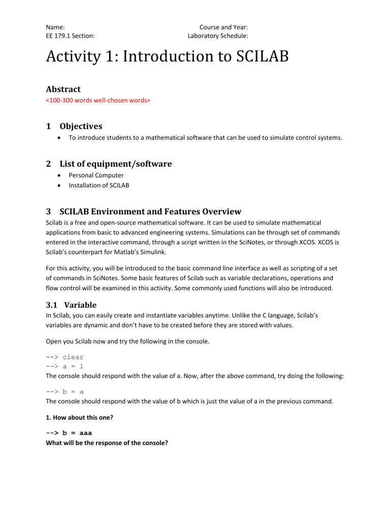
Name:
EE 179.1 Section:
Course and Year:
Laboratory Schedule:
Activity 1: Introduction to SCILAB
Abstract
<100-300 words well-chosen words>
1 Objectives

To introduce students to a mathematical software that can be used to simulate control systems.
2 List of equipment/software


Personal Computer
Installation of SCILAB
3 SCILAB Environment and Features Overview
Scilab is a free and open-source mathematical software. It can be used to simulate mathematical
applications from basic to advanced engineering systems. Simulations can be through set of commands
entered in the interactive command, through a script written in the SciNotes, or through XCOS. XCOS is
Scilab’s counterpart for Matlab’s Simulink.
For this activity, you will be introduced to the basic command line interface as well as scripting of a set
of commands in SciNotes. Some basic features of Scilab such as variable declarations, operations and
flow control will be examined in this activity. Some commonly used functions will also be introduced.
3.1 Variable
In Scilab, you can easily create and instantiate variables anytime. Unlike the C language, Scilab’s
variables are dynamic and don’t have to be created before they are stored with values.
Open you Scilab now and try the following in the console.
--> clear
--> a = 1
The console should respond with the value of a. Now, after the above command, try doing the following:
--> b = a
The console should respond with the value of b which is just the value of a in the previous command.
1. How about this one?
--> b = aaa
What will be the response of the console?
Name:
EE 179.1 Section:
Course and Year:
Laboratory Schedule:
Since aaa has not been assigned a value yet, it still does not exist.
Another convenient feature of Scilab is that you can assign any datatype to a variable even after you had
previously assigned a different datatype. For example:
--> b = 1
--> b = “Hi, this is a string”
--> b = [“this”,”is”, “a”, “vector/array”]
These commands will not produce an error. The datatype of the variables in Scilab adapt to whatever
value you store in it.
You may have noticed that the last command is an array. Arrays in Scilab are values enclosed in “[“ and
“]” with values separated by spaces or commas. You can also create a matrix by separating rows with a
semicolon.
--> an_array = [1, 3, 4]
--> a_matrix = [1, 2; 4, 5]
𝟏 𝟐 𝟑
2. What will you enter in the command line if you want to assign a_matrix with [𝟒 𝟓 𝟔]?
𝟕 𝟖 𝟗
You can easily declare an array of sequence of numbers using “:”
--> 1:10
// returns an array of numbers from 1 to 10 with an
interval of 1
--> 1:2:10
// returns an array of numbers from 1 to 10 with an
interval of 2
3.1.1 Polynomial
You can easily create polynomial using the poly function read the help file for different methods of using
the poly function. The simplest way is the following:
--> s= poly(0,’s’)
//this assign polynomial s^1 to the variable s.
Now you can manipulate this variable similar to number.
3. Write the result of (s^2+2*s+1)/(s+1) as shown in the console.
3.2 Operators
Scilab has a lot of operators in addition to basic arithmetic operations. Since Scilab operates on matrices
by default, basic arithmetic operations are applied on matrices.
Operator
+
*
/
Description
Matrix addition
Matrix subtraction
Matrix Multiplication
Matrix division. 𝐴/𝐵 = 𝐴 ∗ 𝐵−1
Name:
EE 179.1 Section:
\
^
‘
Course and Year:
Laboratory Schedule:
Matrix back-division. 𝐴\𝐵 = 𝐴−1 ∗ 𝐵
Matrix exponential.
Transpose
If you want element-wise operation using those operators, the operator is preceded with a “.”
--> a = [1, 2; 3, 4]
--> b = [3, 4; 5, 6]
--> a + b
ans =
4.
6.
8.
10.
4. Do a matrix multiplication and element-wise multiplication on a and b. What are the results? Are
the results equal?
5. What is the result of a’?
Accessing an element in an array or matrix is by calling the variable with a parenthesis. For example, to
access the 1st element of b:
--> b(1) //this will return 3. Matrix b is treated as a vector reading
top to bottom starting from the left.
This is the same as
--> b(1,1) //accessing element in column 1 row 1. First index is for
the row, the second is for the column.
You can use the $ to indicate the index of the last element.
--> b(1,$) //returns the last element of the first row.
Sub-matrices can be extracted by putting an array or matrix as index. The content of the matrix index
will be the rows/columns that will be included in the sub-matrix. You can use “:” to include all elements
on that row/column.
--> c = [1, 2 ,3; 4, 5, 6; 7, 8, 9]
--> d = c([1,3],[1,2])
ans =
1.
2.
3.
8.
--> e = c(:,1) //returns all the rows in the first column.
6. What is the result of c(1:3,$)?
Name:
EE 179.1 Section:
Course and Year:
Laboratory Schedule:
3.3 Flow Control
The flow control in Scilab can be done with if then/else statements, select/case , return, for loop, do and
while loops. In addition, keywords such as break, continue, pause, abort are also useable to alter the
flow of a set of Scilab commands. The syntax for this is in described in detailed in the Help menu of
Scilab. To access the Help, type help in the command line or click the help button in the menu bar.
3.4 Functions in Scilab
You can create a reuseable set of commands as a function in Scilab. The basic syntax is the following:
FUNCTION [y1,…, yn]= functionname(x1, …, xm)
//some statements or commands here
ENDFUNCTION
3.4.1 Some of the commonly used functions in Scilab
Refer to the Help menu for details
1.
2.
3.
4.
5.
6.
7.
8.
9.
10.
11.
12.
13.
14.
15.
16.
17.
18.
19.
20.
plot – used to plot expressions in Scilab.
poly – function to create a polynomial.
roots – Solve the roots of a polynomial
coeff – extract the coefficients of a polynomial.
evstr - evaluate a string of Scilab statements or commands
csim – Simulation of a linear system. (time response)
ones – Generate a matrix of ones
zeros – Generate a matrix of zeroes
rand – generate a matrix of random values
eye – generate an identity matrix.
inv – inverse of a matrix
diag – extract the diagonal of matrix
abs – absolute value
real, imag, complex – for complex numbers
conj – conjugate of a complex
pfss – partial fraction expansion of a give transfer function
syslin – system linear definition
ss2tf – State-space representation to transfer function conversion
tf2ss – Transfer function to state-space representation
ssrand – random system generator.
3.5 Batch Commands or Scripting
Scilab has an integrated text editor called SciNotes for creating and editing Scilab scripts. A set of
commands or statements can be written in a Scilab script that can be ran or executed in a single action.
Name:
EE 179.1 Section:
Course and Year:
Laboratory Schedule:
SciNotes has some advance text editing functionalities for coding like parenthesis matching and syntax
highlighting. Open Scinote by clicking the notebook icon below the menu bar.
After opening the SciNotes, do the following:
7. Write the following in the editor:
a = [0:0.1:2*%pi]
b = “this is executed after a=1”
plot(a,sin(2*a))
//end
What is the result or the behavior of the above statements in the console after executing the script?
8. Write a function called myfunct that accepts two parameters A and B. The function will return the
result of (A+B)*B. Execute the script what is the result?
9. Call the function you created in #8 and pass as parameters the values 3 and 9. What is the result?
10. What will your function return if the parameters are [1,2,3] and [4; 6;7]?
11. How about [1, 2, 3 ; 3, 5, 1; 5 6 -1] and [3, -1, 4 ; -3, 5, 1; -5 6 -1]?
12. Do you have to re-execute your function from SciNotes? Why?
3.6 Answers to Questions
4 Conclusion
<Write your conclusion about the things you did in this lab>