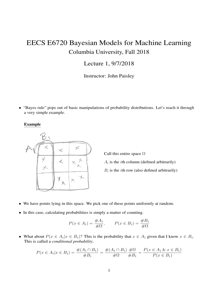
EECS E6720 Bayesian Models for Machine Learning
Columbia University, Fall 2018
Lecture 1, 9/7/2018
Instructor: John Paisley
• “Bayes rule” pops out of basic manipulations of probability distributions. Let’s reach it through
a very simple example.
Example
Call this entire space Ω
Ai is the ith column (defined arbitrarily)
Bi is the ith row (also defined arbitrarily)
• We have points lying in this space. We pick one of these points uniformly at random.
• In this case, calculating probabilities is simply a matter of counting.
P (x ∈ A1 ) =
#A1
,
#Ω
P (x ∈ B1 ) =
#B1
#Ω
• What about P (x ∈ A1 |x ∈ B1 )? This is the probability that x ∈ A1 given that I know x ∈ B1 .
This is called a conditional probability.
P (x ∈ A1 |x ∈ B1 ) =
#(A1 ∩ B1 )
#(A1 ∩ B1 ) #Ω
P (x ∈ A1 & x ∈ B1 )
=
=
#B1
#Ω
#B1
P (x ∈ B1 )
1
• We’ve simply multiplied and divided by the same thing, but already we’ve made a general statement.
A more general statement
• Let A and B be two events, then
P (A|B) =
P (A, B)
P (B)
⇒
P (A|B)P (B) = P (A, B)
• We have some names for these terms,
P (A|B) : conditional probability distribution
P (A, B) : joint probability distribution
P (B) : marginal probability distribution
• This last one could be tricky, since it’s also just “the probability of B.” However, we can use the
same counting approach as before to interpret P (B) as a distribution arrived at by integrating (or
marginalizing) something out. From the previous example,
#B
P (B) =
=
#Ω
P3
i=1
3
3
X
X
#(Ai ∩ B)
#(Ai ∩ B)
=
=
P (Ai , B)
#Ω
#Ω
i=1
i=1
• Side note: In general, the summation and each Ai have a very strict requirement. Each Ai has to
be disjoint (no overlaps) and the union of all the Ai has to equal the intersection of Ω with B.
Getting to Bayes rule
• We’re a few easy steps away. We showed that
P (A, B) = P (A|B)P (B)
By symmetry we could just as easily have shown that
P (A, B) = P (B|A)P (A)
And therefore,
P (A|B) =
P (B|A)P (A)
P (B|A)P (A)
P (B|A)P (A)
= P
= P
P (B)
i P (Ai , B)
i P (B|Ai )P (Ai )
• This equality is called Bayes rule. As you can see, it has a few ways it can be written.
Bayes rule
• And so we have that P (A|B) =
P (B|A)P (A)
P (B)
2
• These values each have a name:
posterior =
likelihood × prior
evidence
• Imagine that we don’t know A, but we get some information about it in the form of B. Bayes
rule tells us a principled way to incorporate this information in our belief about A.
Example (medical test)
• We have two binary values, A and B:
(
1 person has disease
A=
0 no disease
(
B=
1 test for disease “positive”
0 test is “negative”
• A person tests “positive” for the disease. What’s the probability he has it?
• We want P (A = 1|B = 1). Does Bayes rule help? Bayes rule says that
P (A = 1|B = 1) =
=
P (B = 1|A = 1)P (A = 1)
P (B = 1)
P (B = 1|A = 1)P (A = 1)
P (B = 1|A = 1)P (A = 1) + P (B = 1|A = 0)P (A = 0)
• Image we can estimate that
P (B = 1|A = 1) = 0.95,
P (B = 1|A = 0) = 0.05,
P (A = 1) = 0.01 = 1 − P (A = 0)
Then plugging in, we have that P (A = 1|B = 1) = 0.16
Continuous space
• We’ve been talking about discrete distributions so far. That is, the number of possible values the
unknowns can take is finite.
• When values are in a continuous space, we switch to continuous distributions.
Example
x ∈ R, p(x) is its density (represented by the switch
to lower case)
R
p(x) ≥ 0 and p(x)dx = 1
R
P (x ∈ A) = A p(x)dx
• The same rules apply as for discrete random variables
3
p(x, y)
,
• p(x|y) =
p(y)
Z
p(y) =
Z
p(x, y)dx,
p(y) =
p(y|x)p(x)dx
• p(x|y)p(y) = p(x, y) = p(y|x)p(x)
• This leads to Bayes rule for continuous random variables
p(y|x) =
p(x|y)p(y)
p(x|y)p(y)
= R
p(x)
p(x|y)p(y)dy
• The difference is that we are dealing with continuous functions.
Bayesian modeling
• Applying Bayes rule to the unknown variables of a data modeling problem is called Bayesian
modeling.
• In a simple, generic form we can write this process as
x ∼ p(x|y) ← The data-generating distribution. This is the model of the data. By model
we mean a probability distribution of how we think the data “got there.” We define this
function, but it has parameters y that we don’t know.
y ∼ p(y) ← The prior distribution on the model parameters (or just model prior). This
is what we think about y a priori. We define this as well.
• The goal is to learn y. Knowing about Bayes rule, we can write that
p(y|x) =
p(x|y)p(y)
∝ p(x|y)p(y)
p(x)
• In the above line, we don’t know p(y|x) and want to calculate it. It answers the question “Having
seen x, what can we say about y?” The right two terms p(x|y)p(y) we do know because we have
defined it. The symbol ∝ is read as “is proportional to.”
• This is the general form of the problems discussed in this class. However, it is non-trivial because
1. p(x|y) can be quite complicated
2. p(y|x) can be intractable because the integral in the normalizing constant doesn’t have a
closed-form solution, thusRrequiring an algorithm to approximate. In other words, we can’t
solve the integral p(x) = p(x|y)p(y)dy.
• These two issues will make up the focus of this class: Defining various models on the structure
of the data-generating phenomenon, and defining inference algorithms for learning the posterior
distribution of that model’s variables. We’ll discuss specific examples to make things concrete,
but really the purpose is to develop a set of techniques that you’ll be able to adapt to new problems
not discussed here.
4
A comment on the notation ∝
• The symbol ∝ can be confusing at first, but it will appear often so it’s good to focus on what it
means at the start. For now, think of y as an unknown model variable whose range of possible
values is in a continuous space. In other words, the posterior p(y|x) is a continuous distribution.
• Think of p(y|x) just as a function of y that is always positive and integrates to 1 over y
• We can also think of the likelihood×prior p(x|y)p(y) as a function of y as well
• Saying p(y|x) ∝ p(x|y)p(y) means that there is some value C such that p(y|x) = Cp(x|y)p(y).
1
so this isn’t that interesting or useful yet.
In fact, we know C = p(x)
• By multiplying by C we’re just scaling up or down one function of y so that it equals
another function of y at all values for y. (Obviously this can only be done if they’re
proportional, hence the symbol ∝.)
• The useful part comes when we multiply by some other number C 0 (often implicitly) so
that p(y|x) 6= C 0 p(x|y)p(y), but still p(y|x) ∝ C 0 p(x|y)p(y).
• Example: Imagine p(x|y) =
1
2
√ 1 e− 2a (x−y)
2πa
1 2
√ 1 e− 2b y .
2πb
and p(y) =
2 − 1 y2
2b
1
p(y|x) ∝ (2π)−1 (ab)−1/2 e− 2a (x−y)
1
1
∝ e− 2a (y
Then
2 −2yx)− 1 y 2
2b
2
We’ve just defined C 0 = (2π)−1 (ab)−1/2 e− 2a x .
• Notice that C 0 is a function of x, but not a function of y. Since we only want the function p(y|x),
C 0 is constant from the perspective of y. Therefore, the implied C 0 can be very complicated.
• To make this even more explicit, notice that
2 − 1 y2
2b
1
p(y|x) = R
(2π)−1 (ab)−1/2 e− 2a (x−y)
1
(2π)−1 (ab)−1/2 e− 2a (x−y)
1
2
2 − 1 y2
2b
1
2
dy
1
2
(2π)−1 (ab)−1/2 e− 2a x e− 2a (y −2yx)− 2b y
=
1 2 R
1
1 2
2
(2π)−1 (ab)−1/2 e− 2a x e− 2a (y −2yx)− 2b y dy
= R
1
2 −2yx)− 1 y 2
2b
1
2 −2yx)− 1 y 2
2b
e− 2a (y
e− 2a (y
dy
• The key is that things cancel in the numerator and denominator. The whole purpose of this is: 1)
it can remove clutter and sometimes make the solution easier to see, 2) it reduces the amount of
stuff you need to write when deriving things. It’s purely something for convenience.
Simple example: beta-Bernoulli model
• We have a sequence of observations X1 , . . . , XN , where Xi = 1 indicates “success” and Xi = 0
indicates “failure.” Think of them as results of flipping a coin.
• We hypothesize that each Xi is generated by flipping a biased coin, where P (Xi = 1|π) = π.
5
• We further assume the Xi are independent and identically distributed (iid). This means the Xi
are conditionally independent given π. Mathematically this means we can write
P (X1 , . . . , XN |π) =
N
Y
P (Xi |π)
i=1
• Since P (Xi |π) = π Xi (1 − π)1−Xi , we can write
P (X1 , . . . , XN |π) =
N
Y
π Xi (1 − π)1−Xi
i=1
• We are interested in the posterior distribution of π given X1 , . . . , XN , i.e.,
P (π|X1 , . . . , XN ) ∝ P (X1 , . . . , XN |π)p(π)
N
Y
∝
π Xi (1 − π)1−Xi p(π)
i=1
• We’ve come across the next significant problem: What do we set p(π) to?
A first try
• Let p(π) = U nif orm(0, 1) ⇒ p(π) = 1(0 ≤ π ≤ 1)
• Then by Bayes rule,
P
p(π|X1 , . . . , XN ) =
π(
i
Xi +1)−1
R1
0
π
P
i
P
(1 − π)(N −
Xi (1
− π)N −
P
i
i
Xi +1)−1
Xi dπ
• The normalizing constant is tricky, but fortunately mathematicians have solved it,
p(π|X1 , . . . , XN ) =
Γ(1 +
P
P
Γ(N + 2)
P
π i Xi +1−1 (1 − π)N − i Xi +1−1
i Xi )Γ(1 + N −
i Xi )
P
(Γ(·) is called the “gamma function”)
• This is a very common distribution called a beta distribution:
Beta(a, b) =
Γ(a + b) a−1
π (1 − π)b−1
Γ(a)Γ(b)
• In the case of the above posterior distribution, a = 1 +
P
i
Xi and b = 1 + N −
P
i
Xi .
• Notice that when a = b = 1, Beta(1, 1) = U nif orm(0, 1) which was the prior we chose.
6
A conjugate prior
• The beta distribution looks a lot like the likelihood term. Also, because it has the U nif orm(0, 1)
distribution as a special case, it would give us a wider range of prior beliefs that we could express.
What if we try the beta distribution as the prior for π?
p(π|X1 , . . . , XN ) ∝ p(X1 , . . . , XN |π)p(π)
i
h P
ih Γ(a + b)
P
a−1
b−1
Xi
N − i Xi
i
π (1 − π)
∝ π
(1 − π)
Γ(a)Γ(b)
∝ π a+
P
i
Xi −1
(1 − π)b+N −
P
i
Xi −1
• We can notice a few things here:
Γ(a+b)
in the last line. This is because it doesn’t depend on π, and so it can
1. I threw away Γ(a)Γ(b)
be absorbed in the normalizing constant. In other words, the normalizing constant is the
integral of the numerator. If we divide the second line by this integral, we can immediately
Γ(a+b)
cancel out Γ(a)Γ(b)
. The result is the third line divided by the integral of the third line. The
only reason to do something like this is for convenience and to make things look simpler.
2. In this case, we know what to divide this
probability distribution on π. The
Pby to make it aP
last line is proportional to a Beta(a + i Xi , b + N − i Xi ) distribution.
• Therefore, p(π|X1 , . . . , XN ) = Beta(a +
P
i
Xi , b + N −
P
i
Xi ).
• Notice that for this problem, when we select the prior p(π) to be a beta distribution, we find that
the posterior distribution is also a beta distribution with different parameters. This is because the
beta distribution is a conjugate prior for this problem.
• We say that a distribution is a “conjugate prior” for a particular variable in a likelihood, or
that it is “conjugate to the likelihood,” if the posterior is in the same distribution family as the
prior, but has updated parameters. Conjugate priors are very convenient, since we only need to
collect sufficient statistics from the data in order to transition from the prior to the posterior.
P For
example, in the problem
above
we
only
need
to
count
the
total
number
of
“successes”
(
i Xi )
P
and “failures” (N − i Xi ).
• will see many conjugate priors in this course and how they can result in fast inference algorithms
for learning models.
What do we gain by being Bayesian?
• For the previous modeling problem with a beta prior, consider the expectation and variance of π
under the posterior distribution.
P
P
P
a + i Xi
(a + i Xi )(b + N − i Xi )
E[π] =
,
V ar(π) =
a+b+N
(a + b + N )2 (a + b + N + 1)
7
• Notice that as N increases,
1. The expectation converges to the empirical success rate.
2. The variance decreases like 1/N , i.e., it’s going to zero.
• Compare this with maximum likelihood, in which we seek a point estimate (on specific value) of
π to maximize the likelihood term only
N
1 X
Xi
π = arg max p(X1 , . . . , XN |π) =
π
N i=1
• The Bayesian approach is capturing our uncertainty about the quantity we are interested in.
Maximum likelihood does not do this.
• As we get more and more data, the Bayesian and ML approaches agree more and more. However,
Bayesian methods allow for a smooth transition from uncertainty to certainty.
8