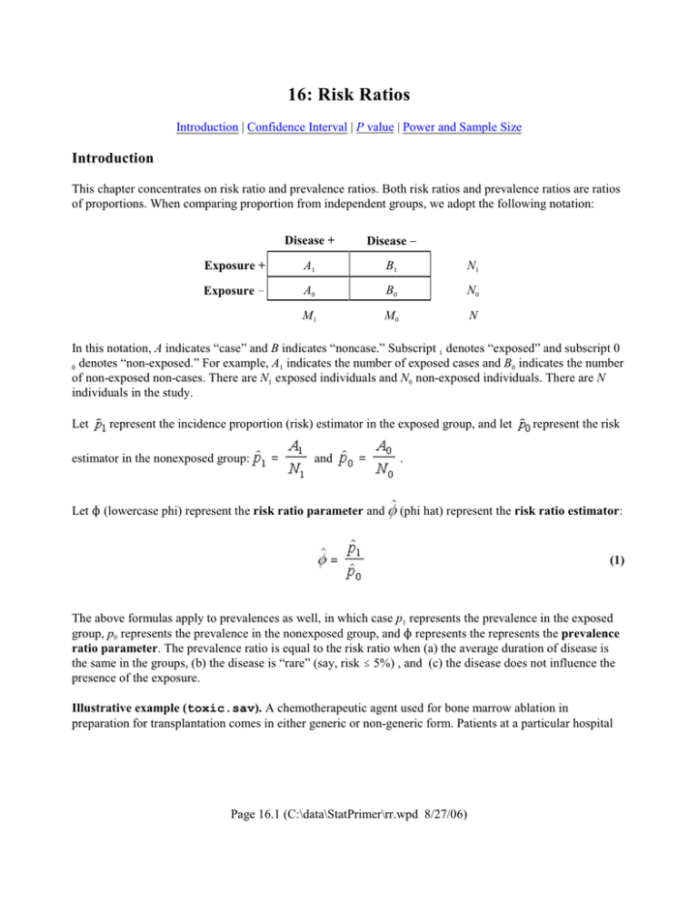
16: Risk Ratios
Introduction | Confidence Interval | P value | Power and Sample Size
Introduction
This chapter concentrates on risk ratio and prevalence ratios. Both risk ratios and prevalence ratios are ratios
of proportions. When comparing proportion from independent groups, we adopt the following notation:
Disease +
Disease -
Exposure +
A1
B1
N1
Exposure !
A0
B0
N0
M1
M0
N
In this notation, A indicates “case” and B indicates “noncase.” Subscript 1 denotes “exposed” and subscript 0
0 denotes “non-exposed.” For example, A1 indicates the number of exposed cases and B0 indicates the number
of non-exposed non-cases. There are N1 exposed individuals and N0 non-exposed individuals. There are N
individuals in the study.
Let
represent the incidence proportion (risk) estimator in the exposed group, and let
estimator in the nonexposed group:
and
Let N (lowercase phi) represent the risk ratio parameter and
represent the risk
.
(phi hat) represent the risk ratio estimator:
(1)
The above formulas apply to prevalences as well, in which case p1 represents the prevalence in the exposed
group, p0 represents the prevalence in the nonexposed group, and N represents the represents the prevalence
ratio parameter. The prevalence ratio is equal to the risk ratio when (a) the average duration of disease is
the same in the groups, (b) the disease is “rare” (say, risk . 5%) , and (c) the disease does not influence the
presence of the exposure.
Illustrative example (toxic.sav). A chemotherapeutic agent used for bone marrow ablation in
preparation for transplantation comes in either generic or non-generic form. Patients at a particular hospital
Page 16.1 (C:\data\StatPrimer\rr.wpd 8/27/06)
received either the generic or non-generic formulation.* The study outcome was cerebellar toxicity. Crosstabulation revealed:
Thus,
,
Toxicity +
Toxicity -
Generic +
11
14
25
Generic -
3
31
34
14
31
59
, and
.
Interpretation: The risk ratio of 4.99 (about 5) indicates that risk in the exposed group is 5-times that of the
non-exposed group. The segment of the risk ratio above (or below) 1 quantifies the relative increase (or
decrease) in risk associated with exposure. For example, the risk ratio of 5 reveals a 5 ! 1.00 = 400(100%) =
400% increase in risk with exposure.
*
Jolson, H. M., Bosco, L., Bufton, M. G., Gerstman, B. B., Rinsler, S. S., W illiams, E., et al. (1992).
Clustering of adverse drug events: analysis of risk factors for cerebellar toxicity with high-dose cytarabine. JNCI, 84,
500-505.
Page 16.2 (C:\data\StatPrimer\rr.wpd 8/27/06)
Confidence Interval for the Risk Ratio
To calculate a 95% confidence interval for the risk ratio parameter, convert the risk ratio estimate to a
natural log (ln) scale. (Use the ln key or “inverse e” key on your calculator.) For the illustrative data, the
natural log of the risk ratio = ln(4.99) = 1.607.
The standard error of the natural log of the risk ratio is
(2)
and a 95% confidence interval for the lnN is
(3)
We then take antilogs of these limits to convert them to a non-logarithmic scale. (The antilog key on your
calculator might be labeled e, for “exponent,” or you might have to use the inverse–lnx key.)
Illustrative example. For the illustrative data,
= 0.5964. A 95% confidence
interval for lnN = 1.607 ± (1.96)(0.5964) = 1.607 ± 1.169 = (0.4381, 2.779). The 95% CI for N = e(0.4381, 2.779)
= (1.55, 16.05), giving us a better idea of what might be in the population. To calculate a 90% confidence
interval, change the 1.96 in formula 3 to 1.645. A 90% confidence interval for lnN= 1.607 ± (1.645)(0.5964)
= 1.607 ± 0.981 = (0.626, 2.588). The 90% confidence interval for N = e (0.626, 2.588) = (1.87, 13.30).
Assumptions: The interpretation of statistics requires assumptions. Distributional assumptions for the above
formulas are based on a normal sampling distribution. Normality can be assumed when expected values in
the table are at least 5. Validity assumptions require no information bias, no selection bias, and no
confounding, as discussed in prior chapters.
Page 16.3 (C:\data\StatPrimer\rr.wpd 8/27/06)
p Value
Chi-Square with Continuity Correction
The test for H0 : N = 1 can be performed with the chi-square test introduced in Chapter 10. That test was
called the Pearsons’s uncorrected chi-square test. We now introduce Yates’ continuity corrected chi-square.
As with the uncorrected chi-square statistic, the continuity corrected chi-square test begins by calculating
expected frequencies under the null hypothesis as product of table margins divided by the total. For the
illustrative data, expected frequencies are:
Disease +
Disease -
Exposure +
5.93*
19.07
25
Exposure -
8.07
25.93
34
14
45
59
The continuity-corrected chi-square statistic is
(4)
where Oi represents the observed frequency in cell i Ei represents the expected frequency, and |Oi ! Ei | is the
absolute value of the difference of the observed and expected. With 2-by-2 tables, this statistic has 1 degree
of freedom. For the illustrative data,
c2 Yates
= (|11!5.93|!.5)2 /5.93 + (|14!19.07|!.5)2 /19.07 + (|3!8.07|!.5)2 /8.07 + (|31!25.93|!.5)2 /25.93
= (|5.07|!.5)2 /5.93 + (|!5.07|!.5)2 /19.07 + (|!5.07|!.5)2 /8.07 + (|5.07|!.5)2 /25.93
= 4.572/5.93 + 4.572/19.07 + 4.572/8.07 + 4.572/25.93
= 3.52 + 1.10 + 2.59 + 0.81
= 8.02.
This statistic has 1 degree of freedom.
Relation between c2 stat with 1 df and the Z distribution. For 2-by-2 cross-tabulated data, you can take the
square root of the chi-square statistic. This is now a P (chi) statistic. The chi-statistic has a standard normal
(z) distribution under H0 and can thus be converted to a two-tailed p value with the two-tailed Z table
available in the back of this Reader. For the illustrative data, Pstat = %(P2 stat) = %8.02 = 2.83. We determine p =
.00465 from the table in the back of the book.
*
The expected frequency in cell A1 = (25)(14)/(59) = 5.93
Page 16.4 (C:\data\StatPrimer\rr.wpd 8/27/06)
Fisher’s Exact Test
Chi-square tests must be avoided when an expected frequency in the 2-by-2 table is less than 5. In such
instances, a procedure based on exact probabilities is needed. One such procedure is Fisher’s test.
Fisher’s exact test is based on summing exact probabilities for table permutations that are more extreme than
current data. We will not cover the calculation method, opting instead for calculation with SPSS, WinPepi, or
EpiCalc2000.
Illustrative example (kxnecro.sav). Data on post-operative colonic necrosis following use of
Kayexelate™ are shown below.*
Disease +
Disease -
Exposure +
2
115
117
Exposure -
0
862
862
2
977
979
Expected frequencies are:
Disease +
Disease -
Exposure +
0.24†
116.76
117
Exposure -
1.76
860.24
862
2
977
979
Because two of cells have expectations that are less than 5, the chi-square test is avoided and Fisher’s exact
test is used. Using WinPepi, we derive a two-tailed Fishers p value of .014.
Computation. In SPSS, click Analyze > Descriptive Statistics > Crosstabs. Select the
exposure variable as the row variable and the disease variable as the column variable. Then click
Statistics button > risk box > OK. To calculate chi-square and Fisher’s test, click the
Statistics button and check the Chi-square box. In WinPepi use COMPARE2.EXE > A or B. In
EpiCalc2000, select Tables > 2-by-2 unstratified.
*
Gerstman, B. B., Kirkman, R., & Platt, R. (1992). Intestinal necrosis associated with
postoperative orally administered sodium polystyrene sulfonate in sorbitol. American Journal of Kidney
Diseases, 20, 159-161.
†
The expected frequency in cell A1 = (117)(2) / (979) = 0.24
Page 16.5 (C:\data\StatPrimer\rr.wpd 8/27/06)
Sample Size Requirements
The sample size requirements of a study of risk ratios can be addressed by considering: (A) the sample size
required for a significant test when a true risk ratio greater of a given magnitude exists at a given significance
level and power or (B) the sample required to satisfy a required precision (i.e., provide a confidence interval
of a given width). Let us consider techniques for (A) before moving to (B).
Recall that the significance level (") of a fixed-level test is the probability of a type I error (false rejection of
the null) and power (1!$) is the probability of avoiding a type II error (false retention of the null). Also
recall that we have two competing hypotheses: H0 : N = 1 versus H1 : N = something else. Let N1 denote this
something else, which we call the expected risk ratio under the alternative hypothesis.
We use WinPepi > COMPARE2.EXE. to calculate results. Click the Sample size menu (on top) and
then choose the Proportions (simple comparisons) option. The desired level of significance
(e.g., " = .05 two-sided), power (e.g., 1!$ = .90), and expected value of the risk ratio under the alternative
hypothesis (e.g., N1 = 2.0) are entered into the program. In addition, the relative sizes of the groups (e.,g.,
N0 /N1 = 1)* must be entered, as must the assumed proportion in the non-exposed group (e.g., p0 = .10).
Clicking “Run” provides results for uncorrected (Pearson’s) and continuity corrected (Yates’) chi-square
testing.
Illustrative example. Using the parenthetical assumptions in the prior paragraph derives the following
output:
Thus, we need a total sample size of 572 when using the continuity corrected test.
*
W inPepi calls the non-exposed group B and exposed group A
Page 16.6 (C:\data\StatPrimer\rr.wpd 8/27/06)