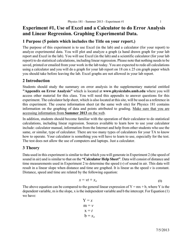
Physics 181 - Summer 2013 - Experiment #1
1
Experiment #1, Use of Excel and a Calculator to do Error Analysis
and Linear Regression. Graphing Experimental Data.
1 Purpose (5 points which includes the Title on your report.)
The purpose of this experiment is to use Excel (in the lab) and a calculator (for your report) to
analyze experimental data. You will plot and analyze a graph (a hand drawn graph for your lab
report and Excel in the lab). You will use Excel (in the lab) and a scientific calculator (for your lab
report) to do statistical calculations, including linear regression. Please note that nothing needs to be
saved, printed or emailed from your work in the lab today. You are expected to redo all calculations
using a calculator and you will do a graph for your lab report on 18 cm x 25 cm graph paper which
you should take before leaving the lab. Excel graphs are not allowed in your lab report.
2 Introduction
Students should study the summary on error analysis in the supplementary material entitled
"Appendix on Error Analysis" which is located at www.physicslabs.umb.edu where you will
access other material for this class. You will need this appendix to answer questions for this
experiment. The calculator help sheet, which is also located at this site, will be used as a reference in
this experiment. The course information sheet (at the same web site) for Physics 181 contains
information on the graphing of data and points attributed to grading. Make sure that you are
accessing information from Summer 2013 on the web.
In addition, students should become familiar with the operation of their calculator to do statistical
calculations, including linear regression. Sources available to learn how to use your calculator
include: calculator manual, information from the Internet and help from other students who use the
same, or similar, type of calculator. There are too many types of calculators for your TA to know
how to operate. Your calculator is something you will have to learn to use, especially for the test.
The test does not allow the use of computers and laptops. Just a calculator.
3 Theory
Data used in this experiment is similar to that which you will generate in Experiment 2 (the speed of
sound in air) and is similar to that on the “Calculator Help Sheet”. Data will consist of distance and
time measurements used in Experiment 2 to determine the speed (v) of sound in air. This data will
result in a linear slope when distance and time are graphed. It is linear as the speed v is constant.
Distance, speed and time are related by the following equation:
x = vt + xo
(1)
The above equation can be compared to the general linear expression of Y = mx + b, where Y is the
dependent variable, m is the slope, x is the independent variable and b the intercept. For Equation (1)
we have:
Y=x
m=v
x=t
b = xo
7/5/2013
2
Linear regression on your calculator, and a graph of distance x versus time t, should generate
information of the form Y = mx + b. In Experiment 2 you will see that the accepted value of the
speed of sound in air (at 25.0oC) is vaccepted = 34.699 cm/ms. 25.0oC is 25.0 degrees Celsius. Note
that cm/ms = centimeter/millisecond and that 1ms = 0.001 seconds = 1x10-3 seconds. And, 1 meter
(m) is equal to 100 centimeters (cm).
Additional distance data will be given for statistical analysis. Once again, students should study the
summary on error analysis at www.physicslabs.umb.edu to attain information on the process of
averaging (statistical mean), determining the standard deviation and calculating the standard
deviation of the mean. Please note that in future experiments, theory information is embedded in the
write-ups. If you do a theory section for your report (which is optional) you may too access the
information through your reading. Your Physics 107 or 113 books are a great source of information
for this lab. This lab is not responsible for the sequence of information taught in these courses.
4 Experimental Apparatus and Procedure
4.1 Experimental Apparatus
The two devices for this experiment are a computer with Microsoft Excel and your
calculator. Your personal calculator is not required in the lab for this experiment, but will be
needed for the laboratory report, and for the rest of the session’s reports, including the lab
test. Computers will not be allowed during the lab test, so experience in the use of your
calculator is very important. Excel is not required once you leave the lab, as your calculator
should be used for laboratory report calculations and questions, as well as calculations you
will do for the pre-lab test. The first pre-lab test will be done for the second experiment. See
the information sheet for information on the pre-lab test. These pre-lab test are located on the
Physics 181 Website. Pre-lab test are due when you come to the lab. Late pre-lab test are not
accepted. They are worth 10 points. Pre-lab test are due when you come to the lab to do the
experiment.
4.2 Experimental Procedure
In this experiment will be present with two sets of data. One set for single variable statistics
(mean, standard deviation and standard deviation of the mean), and a second set of date for
multiple variable statistics using linear regression. You will use Excel in the lab to analyze
these data sets, and your calculator to analyze these data sets for your first lab report. Please
note that Experiment 2 will include single and multiple variable statistics.
5 Data (15 points)
5.1 Single Variable Statistics
The following data will be entered into Excel during the lab. Your Excel sheet should
resemble Figure 1 which contains this data. This distance x measurement data is similar to
what you will be collecting in the second part of Experiment 2. Note that all data is collected
with a precision of one hundredth of a centimeter, or, two places after the decimal point. For
your report (and information you are required to enter into your data section) the uncertainty,
or error, associated with a single measurement of distance is ± x = 0.05 cm. This error value
will be explained to you during Experiment 2 when you will take measurements of distance.
Physics 181 - Summer 2013 - Experiment #1
3
The following distance data will be used for statistical analysis.
Distance (cm)
60.25
60.20
60.23
60.21
60.24
Figure 1. Distance x measurements entered in Excel.
5.2 Multiple Variable Statistics
The following data for distance and time (which you will too be collecting in Experiment 2)
will be entered into Excel for this experiment. See Figure 2. This is the data you will be
using to do linear regression.
Time (ms)
0.50
1.00
1.50
2.00
2.50
3.00
Distance (cm)
8.07
25.30
42.72
60.22
77.38
94.83
Figure 2. Distance x and time t measurements entered in Excel.
The error in time will not be included in this experiment so you will not enter it into your
data section. Your error (uncertainty) associated with the distance x measurement is ±x =
0.05 cm. This is entered into the data section. Please note that the measurement in time is the
independent variable, and the distance measurement is the dependent variable. When
entering data in Excel and calculators, the independent variable, here time, is usually entered
first.
7/5/2013
4
In Figure 2, time is entered before distance as this column is selected first when choosing
data to do a graph in Excel. Again, time is the independent variable and is entered before
entering the dependent variable in most calculators.
Data in 5.1 and 5.2 should be entered into your lab report in tables similar to the above.
Enter errors in each measurement in this section of your report. Here, just the errors in the
two distance measurements: ± x = 0.05 cm. You may copy and paste tables from Excel into
your report. Feel free to create Excel files for these reports on your personal computer or
laptop. Remember, you may not bring laptops to the lab test.
6 Calculations and Analysis (25 Points) and Graph (10 Points)
1.
Enter, in Excel, your data for 5.1. Your Excel sheet should reflect Figure 1. Use
Excel functions (fx) to calculate the mean (AVERAGE) and standard deviation
(STDEV.S or STDEV). These functions are used in Microsoft Office 2010. Your
Excel sheet should resemble Figure 3 when calculations are completed.
Figure 3. Average (mean) and standard deviation Excel calculations.
In Figure 3, use the correct function in Excel to set rows 8 and 9 (column A) to three
numbers after the decimal point. The correct units are entered in column B. Your
Excel sheet has to be the same for this experiment in the lab. Refer to the “Calculator
Help Sheet” for information how your results for the mean and standard deviation
should be entered into your lab report.
2.
Use the Excel = function to calculate the standard deviation of the mean (SDM) for
the distance x data. The standard deviation of the mean is given as:
SDM =
s
N
where s is the standard deviation and N is the number of measurements. For this
calculation, N equals 5 data points of distance x. Your final results should resemble
Figure 4.
Physics 181 - Summer 2013 - Experiment #1
5
Figure 4. SDM calculation using Excel.
As indicated above column C in Figure 4, SDM “=A9/(5)^.5”. Note that (5)^.5 is the
square root of 5. You may also use SDM “=A9/SQRT(5)” in Excel.
Most of your calculations in this lab will use Excel and the fx= function. Refer to the
“Calculator Help Sheet” for information how your results for the standard deviation
of the mean should be entered into your lab report. For your lab report, use your
calculator to find the mean, standard deviation and the standard deviation of the
mean. You are required to show the formula for the SDM, and its calculation, in your
reports. Use of an equation editor is not required. Formulas and calculations should
be written neatly with pen or pencil, unless you want to use an equation editor or can
be neatly typed in. In your lab report, you would enter the SDM in Figure 4 as SDM
= 0.009cm = 0.01cm. Again, refer to the “Calculator Help Sheet” on this.
From Figure 4 we have the average experimental value of distance x = 60.23 ± 0.01
cm. This should be entered into your lab report. This result indicates our best
estimate of x (the average of 60.23 cm) which is known with an uncertainty of ± 0.01
cm (the SDM). Note that our uncertainty, or error, from a single measurement of x is
± 0.05 cm. The use of multiple measurements of x has increased our precision, or
reliability, in its measurement to ± 0.01 cm which yields a percent fractional error of
0.02%.
3.
For your lab report, plot a graph of distance x (cm) versus time t (ms). In class, you
plot this graph using Excel. For your lab report, you are required to plot this
graph by hand using cm-mm graph paper. This graph will be worth 10 points.
Since the speed is constant, the graph of x vs. t should be a straight line. Use a clear
plastic ruler to draw, on your graph, a thin straight line which best accommodates the
linear data points. The origin of this graph should be 0.00 on both axes and at the
most lower left hand corner. It is suggested that you use the 25 cm side for distance
and the 18 cm side for time. Your distance scale will be 1 cm on the graph = 4 cm of
distance measured (1 cm = 4 cm). Refer to Figure 5.
The following are requirements for graphs, and points associated with each, for your
report. Read the information sheet for additional information on doing graphs.
1. You must use 75%, or more, of the graph area.
2 points
7/5/2013
6
2.
3.
4.
5.
6.
7.
8.
You must use a pencil.
Title your graph
Axes must have name and units
Show the scale used for each axis (1cm = x units)
Show the data points and linear line of best fit
Equation of the line (Y = mx + b)
Calculation of slope from non-data points (xa, ya)
1 point
1 point
1 point
1 point
2 points
1 point
1 point
Graphs should be used as a device to detect data points which fail to be linear with
the rest of your data. Incorrect data should not be used when drawing the line of best
fit and excluded when entering data into your calculator to determine the slope and
intercept (linear regression).
Your Excel graph in class should reflect Figure 5. This graph resembles the one on
the “Calculator Help Sheet”. The data is slightly different.
Figure 5. Excel graph of distance x versus time t.
In Figure 5, the slope m is 34.717 cm/ms and the intercept b is -9.334 cm (a negative
value). The time unit of ms (millisecond) is equal to .001 seconds or 1.00x10 -3
seconds. Note that 1 meter is equal to 100 centimeters (cm). In Figure 5, the R2 value
Physics 181 - Summer 2013 - Experiment #1
7
is called the linear coefficient of determination. The more linear your data, the closer
this value is to 1. You should always show this coefficient when calculating a graph
in Excel and doing linear regression on your calculator. This value should always
have four numbers after the decimal point. For Figure 5, R2 = 1.0000.
4.
For your Excel work, calculate the percent error between the experimental value for
the speed of sound in air (vexperimental = 34.717 cm/ms) and the accepted value of the
speed of sound in air (vaccepted = 34.699 cm/ms):
% error = (| vexperimental – vaccepted | / | vaccepted |) (100%)
The percent error is a useful way to measure accuracy. Do this for your Excel value
in the lab (Figure 5).
5.
For your lab report, use the linear regression function on your calculator to calculate
the slope m, intercept b and linear coefficient of determination R2 of the data in
Figure 2. This figure presents time and distance data. Refer to the “Calculator Help
Sheet” for information how a calculator may present Y = mx + b.
6.
For your lab report, use results from part 5 above and Y = mx +b and enter your
values into Equation (1), x = vt + xo. Enter the appropriate units for each term.
7.
For your lab report, calculate the slope and intercept on your hand drawn graph. This
calculation should be done on the graph. Calculate this slope using 2 non-data points
(ta, xa) and (tb, xb). Actual data points should not be used as the line of best fit does
not necessarily pass through them.
To compute the slope of your straight line fit, choose two points (call these a and b)
on the straight line graph and determine their coordinates. These two points should
not be actual data points from your experiment, but information produced by the line
which best fits your data. Coordinates, of the form (ta, xa) and (tb, xb), should be
written on your graphs next to the points on the line of best fit. For simplicity, choose
data points so that the values at point b are much larger than point a.
The slope (m) and the intercept (b) are calculated as:
Slope m =
xb  xa
t b  ta
Intercept b = xa – mta = xa – (
xb  xa
)ta
tb  ta
8.
For your lab report, use your results from part 7 above and enter your results for Y =
mx + b in to Equation (1), x = vt + xo. Enter the appropriate units for each term.
9.
Calculate the percent error between the experimental value for the speed of sound in
air and the accepted value of the speed of sound in air for both your linear regression
value of the slope on your calculator and for the one from your graph’s slope. These
two % errors should be in your lab report. Again, vaccepted = 34.699 cm/ms.
% error = (| vexperimental – vaccepted | / | vaccepted |) (100%)
7/5/2013
8
The percent error is a useful to measure the accuracy of your experimental results.
7 Questions (40 Points for this experiment)
1.
An experiment is done using a two meter long metric ruler to make 10
measurements. Statistical analysis yields a distance mean of 115.25 cm and a
standard deviation of 0.15 cm. The experiment is repeated with 100 measurements.
This yields a distance mean of 114.15 cm and a standard deviation of 0.07 cm. Based
on these results, which average distance is more precise and why? See the "Appendix
on Error Analysis” at www.physicslabs.umb.edu to help in answering this question.
(6 Points)
2.
Calculate the SDM for both sets of data in question 1. Show your calculations. (6
Points)
3.
Calculate the percent fractional errors (PFE) for both measurements in question 1
using the SDM values from question 2. See the "Appendix on Error Analysis” for
information on calculating the PFE. Show your calculations. Indicate which data set,
10 measurements or 100 measurements, has the lowest PFE. (6 Points)
\
4.
Repeat question 3 above and use the error value 0.05 cm instead of the SDM. x =
0.05 cm is the error associated with each single measurement of distance. (6 Points)
5.
Another student performs the same experiment in question 1 and has a distance mean
of only 15.61 cm and not 115.61 cm. What type of “error” should be used to explain
this 100.00 cm reduction in distance in using the measuring device: random,
systematic or personal? (6 Points)
6.
Data in the table below is entered into a calculator and a coefficient of determination
of R2 = 0.9846 is calculated. What data point in this table should be excluded to
improve the value of the linear coefficient of determination R2? (6 Points)
7.
Calculate the linear coefficient of determination R2 in the above table with the
incorrect data excluded. Answer should have four numbers after the decimal
point. When doing your lab report, always enter the linear coefficient of
determination to four numbers after the decimal point. (4 Points)
Physics 181 - Summer 2013 - Experiment #1
9
Conclusion (5 Points)
This section should have a clear statement of the results of the experiment and the extent to which
the results are in agreement with the theory being tested. Use percent error to compare your
experimental result to the accepted or theoretical value. If percent error was done earlier, you are
still required to do it in this section.
To make this comparison meaningful, you should include the impact of the experimental error on
your results. This includes errors in plotting and reading linear graphs when determining their slope
and intercept. Possible systematic and procedural (personal) errors should be included. Please
include a statement of what you have learned, a critique of the experiment, and any suggestions you
have which you think could improve the experiment or the lab handout.
7/5/2013