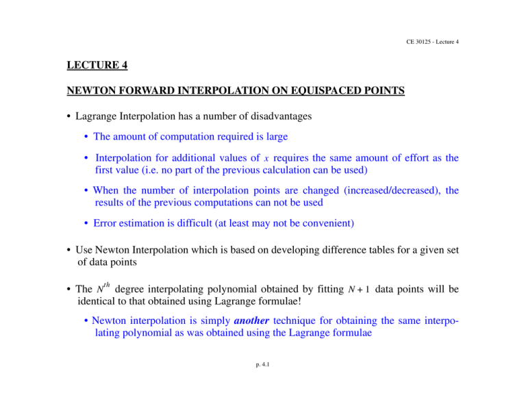
CE 30125 - Lecture 4
LECTURE 4
NEWTON FORWARD INTERPOLATION ON EQUISPACED POINTS
• Lagrange Interpolation has a number of disadvantages
• The amount of computation required is large
• Interpolation for additional values of x requires the same amount of effort as the
first value (i.e. no part of the previous calculation can be used)
• When the number of interpolation points are changed (increased/decreased), the
results of the previous computations can not be used
• Error estimation is difficult (at least may not be convenient)
• Use Newton Interpolation which is based on developing difference tables for a given set
of data points
• The N th degree interpolating polynomial obtained by fitting N + 1 data points will be
identical to that obtained using Lagrange formulae!
• Newton interpolation is simply another technique for obtaining the same interpolating polynomial as was obtained using the Lagrange formulae
p. 4.1
CE 30125 - Lecture 4
Forward Difference Tables
• We assume equi-spaced points (not necessary)
f
f2 = f(x2)
f1 = f(x1)
f3 = f(x3)
f0 = f(x0)
x0
x1
x2
x3
0
1
2
3
fN = f(xN )
x
xN
N (i)
h = interval size
• Forward differences are now defined as follows:
0 fi  fi
(Zeroth order forward difference)
f i  f i + 1 – f i
(First order forward difference)
p. 4.2
CE 30125 - Lecture 4
2
 f i  f i + 1 – f i
(Second order forward difference)
2
 fi =  fi + 2 – fi + 1  –  fi + 1 – fi 
2
 f i = f i + 2 – 2f i + 1 + f i
3
2
2
 fi   fi + 1 –  fi
(Third order forward difference)
3
 f i =  f i + 3 – 2f i + 2 + f i + 1  –  f i + 2 – 2f i + 1 + f i 
3
 f i = f i + 3 – 3f i + 2 + 3f i + 1 – f i
k
 fi = 
k–1
fi + 1 – 
k–1
fi
(kth order forward difference)
• Typically we set up a difference table
p. 4.3
CE 30125 - Lecture 4
2
3
4
i
fi
f i
 fi
 fi
0
fo
f o = f 1 – f o
 f o = f 1 – f o
2
 fo =  f1 –  fo
1
f1
f 1 = f 2 – f 1
 f 1 = f 2 – f 1
2
 f1 =  f2 –  f1
2
f2
f 2 = f 3 – f 2
 f 2 = f 3 – f 2
3
f3
f 3 = f 4 – f 3
4
f4
 fi
3
2
2
3
2
2
4
3
3
 fo =  f1 –  fo
2
• Note that to compute higher order differences in the tables, we take forward differences
of previous order differences instead of using expanded formulae.
• The order of the differences that can be computed depends on how many total data
points, x o  x N , are available
th
• N + 1 data points can develop up to N order forward differences
p. 4.4
CE 30125 - Lecture 4
Example 1
• Develop a forward difference table for the data given
i
xi
fi
f i
 fi
2
 fi
3
 fi
4
 fi
0
2
-7
4
5
5
3
1
1
4
-3
9
10
8
4
2
6
6
19
18
12
3
8
25
37
30
4
10
62
67
5
12
129
p. 4.5
5
CE 30125 - Lecture 4
Deriving Newton Forward Interpolation on Equi-spaced Points
f(x)
f2
f3
f1
fN
f0
x0
x1
x2
x3
xN
x
• Summary of Steps
• Step 1: Develop a general Taylor series expansion for f  x  about x o .
• Step 2: Express the various order forward differences at x o in terms of f  x  and its
derivatives evaluated at x o . This will allow us to express the actual derivatives evaluated at x o in terms of forward differences.
• Step 3: Using the general Taylor series expansion developed in Step 1, sequentially
substitute in for the derivatives evaluated at x o in terms of forward differences (i.e.
substitute in the expressions developed in Step 2).
p. 4.6
CE 30125 - Lecture 4
Step 1
• The Taylor series expansion for f  x  about x o is:
df
f  x  = f  x o  +  x – x o  -----dx
2
x = xo
1
2d f
+ -----  x – x o  -------22!
dx
3
x = xo
1
3d f
+ -----  x – x o  -------33!
dx
+ O  x – xo 
4
x = xo

1
1
2 2
3 3
4
1
f  x  = f o +  x – x o f o + -----  x – x o  f o + -----  x – x o  f o + O  x – x o 
2!
3!
Step 2a
1
• Express first order forward difference in terms of f o , f o  
f o  f 1 – f o
• However since f 1 = f  x 1  , we can use the Taylor series given in Step 1 to express f 1 in
terms of f o and its derivatives:
1
1
2 2
3 3
4
1
f 1 = f o +  x 1 – x o f o + -----  x 1 – x o  f o + -----  x 1 – x o  f o + O  x 1 – x o 
2!
3!
p. 4.7
CE 30125 - Lecture 4
• We note that the spacing between data points is h  x 1 – x o :
1 2 2  1 3 3
1
4
f 1 = f o + hf o + ----- h f o + ----- h f o + O  h 
2!
3!
• Now, substitute in for f 1 into the definition of the first order forward differences
1 2 2 1 3 3
4
1
f o = f o + hf o + ----- h f o + ----- h f o + O  h  – f o
2!
3!

1
fo
f o 1  2  1 2  3 
3
= -------- – ----- hf o – ----- h f o – O  h 
3!
h
2!
• Note that the first order forward difference divided by h is in fact an approximation to
the first derivative to O  h  . However, we will use all the terms given in this sequence.
p. 4.8
CE 30125 - Lecture 4
Step 2b
1
• Express second order forward difference in terms of f o f o  
2
 f o  f 2 – 2f 1 + f o
• We note that f 1 = f  x 1  was developed in T.S. form in Step 2a.
• For f 2 = f  x 2  we use the T.S. given in Step 1 to express f 2 in terms of f o and derivatives of f evaluated at x o
1
1
2 2
3 3
4
1
f 2 = f o +  x 2 – x o f o + -----  x 2 – x o  f o + -----  x 2 – x o  f o + O  x 2 – x o 
2!
3!
• We note that x 2 – x o = 2h
4 2 2 8 3 3
1
4
f 2 = f o + 2hf o + ----- h f o + ----- h f o + O  h 
2!
3!
p. 4.9
CE 30125 - Lecture 4
• Now substitute in for f 2 and f 1 into the definition of the second order forward difference
operator
2
2 2 4 3 3
4
1 
 f o = f o + 2hf o + 2h f o + --- h f o + O  h 
3
2 2 1 3 3
4
1
– 2f o – 2hf o – h f o – --- h f o + O  h  + f o
3

2
fo
2
 fo
2
3
= --------- – hf o + O  h 
2
h
2
• Note that the second order forward difference divided by h is in fact an approximation
2
to f o to O  h  . However, we will use all terms in the expression.
p. 4.10
CE 30125 - Lecture 4
Step 2c
1 
• Express the third order forward difference in terms of f o f o 
3
 f o  f 3 – 3f 2 + 3f 1 – f o
• We already developed expressions for f 2 and f 1 .
• Develop an expression for f 3 = f  x 3  using the T.S. in Step 1
1
1
2 2
3 3
4
1
f 3 = f o +  x 3 – x o f o + -----  x 3 – x o  f o + -----  x 3 – x o  f o + O  x 3 – x o 
2!
3!
• Noting that x 3 – x o = 3h
1 9 2 2 9 3 3
4
f 3 = f o + 3hf o + --- h f o + --- h f o + O  h 
2
2
p. 4.11
CE 30125 - Lecture 4
• Substituting in for f 3 , f 2 and f 1 into the definition of the third order forward difference
formula.
3
4
1  9 2 2 9 3 3
 f o = f o + 3hf o + --- h f o + --- h f o + O  h 
2
2
4
 1  12 2  2  24 3  3 
– 3f o – 6hf o – ------ h f o – ------ h f o + O  h 
2
3!
3 3 3
4
1 3 2 2 
+ 3f o + 3hf o + --- h f o + ----- h f o + O  h  – f o
2
3!

3
3 3
 fo = h fo + O  h 
4

3
fo
3
 fo
= --------- + Oh
3
h
• The third order forward difference divided by h 3 is an O(h) approximation to f o3 
p. 4.12
CE 30125 - Lecture 4
Step 3a
• Consider the general T.S. expansion presented in Step 1 to define f  x  and substitute in
for f o1  using the result in Step 2a.
• Note that now we are not evaluating the T.S. at a data point but at any x
f o 1  2  1 2  3 
3
f  x  = f o +  x – x o  -------- – ----- hf o – ----- h f o – O  h 
3!
h 2!
1
1
2 2
3 3
4
+ -----  x – x o  f o + -----  x – x o  f o + O  x – x o 
3!
2!

x – xo
1
2 2
f  x  = f o + -------------f o + -----  –  x – x o h +  x – x o  f o
2!
h
1
2
3 3
4
+ -----  –  x – x o h +  x – x o  f o + O  h 
3!
p. 4.13
CE 30125 - Lecture 4
Step 3b
2
• Substitute in for f o
using the expression developed in Step 2b.
2
x – xo
1
3
2  fo
2
f  x  = f o + -------------f o + -----  –  x – x o h +  x – x o   --------–
hf
+
O

h

o
2
2!
h
h
1
2
3 3 
4
+ -----  –  x – x o  h +  x – x o  f o + O  h 
3!

2
x – xo
1  x – xo   x – xo 
2
f  x  = f o + -------------f o + ----- – ------------------ + --------------------  fo
2
2!
h
h
h
1
2
3
2
4
3
+ -----  2  x – x o h +  x – x o  – 3  x – x o  h  f o + O  h 
3!
p. 4.14
CE 30125 - Lecture 4
Step 3c
3
• Substitute in for f o
from Step 2c
2
 x – xo 
1  x – xo   x – xo 
2
f  x  = f o + ------------------f o + ----- – ------------------ + --------------------  fo
2
h
h
2!
h
3
2
3
2  fo
4
1
+ -----  2  x – x o h +  x – x o  – 3  x – x o  h  --------- + O h
3
3!
h
• Re-arranging the terms in brackets:
2
f o 1
 fo
f  x  = f o +  x – x o  -------- + -----  x – x o   – h +  x – x o   --------2
h
2!
h
3
 fo
1
2
2
4
+ -----  x – x o   2h +  x – x o  – 3  x – x o h  --------+
O

h

+ HOT
3
3!
h

p. 4.15
CE 30125 - Lecture 4
2
f o 1
 fo
f  x  = f o +  x – x o  -------- + -----  x – x o   x –  x o + h   --------2
h
2!
h
3
 fo
1
4
+ -----  x – x o    x –  x o + h    x –  x o + 2h    --------+
O

h

+ HOT
3
3!
h
• Also considering higher order terms and noting that x o + h = x 1 , x o + 2h = x 2
and
fx = gx + ex 
2
f o 1
 fo
g  x  = f o +  x – x o  -------- + -----  x – x o   x – x 1  ---------2
h
2!
h
3
 fo
1
+ -----  x – xo   x – x 1   x – x2  ---------3
3!
h
N
 fo
1
+  + ------  x – x o   x – x 1   x – x 2   x – x N – 1  ----------N
N!
h
th
• This is the N degree polynomial approximation to N + 1 data points and is identical to that derived for Lagrange interpolation or Power series (only the form in
which it is presented is different).
p. 4.16
CE 30125 - Lecture 4
• Note that the N + 1 data point are exactly fit by g  x 
g  xo  = fo
f1 – fo
f1 – fo
g  x 1  = f o +  x 1 – x o  -------------- = f o + h  -------------- = f 1
 h 
h
f1 – fo
1
1
g  x 2  = f o +  x 2 – x o   -------------- + ---  x 2 – x o   x 2 – x 1  ----2-  f 2 – 2f 1 + f o 
 h  2
h

2h
 2h h
g  x 2  = f o + ------  f 1 – f o  + -------------  f 2 – 2f 1 + f o 
2
h
2h

g  x 2  = f o + 2f 1 – 2f o + f 2 – 2f 1 + f o = f 2
• In general
g  xi  = fi
i = 0 N
p. 4.17
CE 30125 - Lecture 4
• It can be readily shown that the error at any x is: (by carrying through error terms in the
T.S.)
 x – x o   x – x 1   x – x N   N + 1 
e  x  = f  x  – g  x  = ------------------------------------------------------------------ f

 N + 1 !
xo    xN
• This error function is identical to that for Lagrange Interpolation (since the polynomial
approximation is the same).
• However we note that f N + 1  x  can be approximated as (can be shown by T.S.)
f
N + 1
N+1
fo

 x o   ----------------N+1
h
• In fact if f  N + 1   x  does not vary dramatically over the interval
f
N + 1
N+1
fo

    ----------------N+1
h
p. 4.18
CE 30125 - Lecture 4
• Thus the error can be estimated as
N+1
 x – x o   x – x 1   x – x N  
fo
e  x   ------------------------------------------------------------------ -----------------N+1
 N + 1 !
h
• Notes
• Approximation for e  x  is equal to the term that would follow the last term in the
N
th
degree polynomial series for g  x 
th
• If we have N + 2 data points available and develop an N degree polynomial approximation with N + 1 data points, we can then easily estimate e  x  . This was not as
simple for Lagrange polynomials since you then needed to compute the finite
difference approximation to the derivative in the error function.
• If the exact function f  x  is a polynomial of degree M  N , then g  x  will be an
(almost) exact representation of f  x  (with small roundoff errors).
• Newton Interpolation is much more efficient to implement than Lagrange Interpolation. If you develop a difference table once, you can
• Develop various order interpolation functions very quickly (since each higher
order term only involves one more product)
• Obtain error estimates very quickly
p. 4.19
CE 30125 - Lecture 4
Example 2
• For the data and forward difference table presented in Example 1.
• (a) Develop g  x  using 3 points ( x o = 2 , x 1 = 4 and x 2 = 6 ) and estimate e  x 
• (b) Develop g  x  using 4 points ( x o = 2 , x 1 = 4 , x 2 = 6 , x 3 = 8 ) and estimate e  x 
• (c) Develop g  x  using 3 different points ( x o = 6 , x 1 = 8 , x 2 = 10 )
(Part a)
• 3 data points
 N = 2
2
f o 1
 fo
g 3  x  = f o +  x – x o  -------- + -----  x – x o   x – x 1  --------2
h
2!
h
with
xo = 2
x1 = 4
x2 = 6
and h = 2
• Note that the “3” designation in g 3  x  indicates N+1=3 data points
p. 4.20
CE 30125 - Lecture 4
2
• f o , f o and  f o are obtained by simply picking values off of the difference table
(across the row i = 0 )
fo = –7
f o = 4
2
 fo = 5
4 1
5
g 3  x  = – 7 +  x – 2  --- + -----  x – 2   x – 4  --2 2!
4
• The error can be estimated as:
 x – xo   x – x1   x – x2  1 3
e 3  x  = -------------------------------------------------------- ----3-  f o
3!
h
3
• Simply substitute in for x o , x 1 , x 2 , h and pick off  f o = 5 from the table in Example 1
x – 2x – 4 x – 6 1
5
e 3  x  = ---------------------------------------------------  ----3-  5 =  x – 2   x – 4   x – 6  -----6
48
2
p. 4.21
CE 30125 - Lecture 4
(Part b)
• 4 data points x o = 2 , x 1 = 4 , x 2 = 6 , x 3 = 8
 N = 3
• Simply add the next term to the series for g 3  x  in Part a:
3
 fo
1
g 4  x  = g 3  x  + -----  x – x o   x – x 1   x – x 2  --------3
3!
h
• We note that the term we are adding to g 3  x  is actually e 3  x 
3
• Pick off  f o = 5 from the table in Example 1 and substitute in
1
5
g 4  x  = g 3  x  + -----  x – 2   x – 4   x – 6   --3!
8
• The error is estimated as
 x – xo   x – x1   x – x2   x – x3  1 4
e 4  x  = --------------------------------------------------------------------------- ----4-  f o
4!
h
3
e 4  x  =  x – 2   x – 4   x – 6   x – 8  --------384
p. 4.22

CE 30125 - Lecture 4
(Part c)
N=2
• 3 data points x o = 6 , x 1 = 8 and x 3 = 10
• We must shift i in the table such that x o = 6 etc.
2
f o 1
 fo
g 3/s  x  = f o +  x – x o  -------- + -----  x – x o   x – x 1  --------2
h
2!
h
2
• Pick off f o , f o and  f o from the same difference table with a shifted index
fo = 6 ,
f o = 19 ,
2
 f o = 18
• Substituting
19 1
18
g 3/s  x  = 6 +  x – 6  ------ + -----  x – 6   x – 8  -----22 2!
2
p. 4.23
CE 30125 - Lecture 4
Newton Backward Interpolation
• Newton backward interpolation is essentially the same as Newton forward interpolation
except that backward differences are used
• Backward differences are defined as:
o
 fi  fi
Zeroth order backward difference
f i = f i – f i – 1
First order backward difference
2
 f i = f i – f i – 1
k
 fi = 
k–1
fi – 
k–1
Second order backward difference
fi – 1
kth order backward difference
p. 4.24
CE 30125 - Lecture 4
th
• For N + 1 data point which are fitted with an N degree polynomial
2
f N 1
 fN
g  x  = f N +  x – x N  ---------- + -----  x – x N   x – x N – 1  ----------2
h
2!
h
3
 fN
1
+ -----  x – x N   x – x N – 1   x – xN – 2  ----------3
3!
h
N
 fN
1
+ ------  x – xN   x – x N – 1   x – x 1  -----------N
N!
h
• Note that we are really expanding about the right most point to the left. Therefore we
must develop f N , f N etc. in the difference table
x0
xN - 1
x1
p. 4.25
xN
CE 30125 - Lecture 4
Newton Interpolation on Non-uniformly Spaced Data Points
• Newton interpolation can be readily extended to deal with non-uniformly spaced data
points
x0
x1
x2
x3
x4
x
• The difference table for non-uniformly spaced nodes is developed and an appropriate
interpolation formula is developed and used
p. 4.26
CE 30125 - Lecture 4
SUMMARY OF LECTURE 4
• Newton formulae can be obtained by manipulating Taylor series
• Newton interpolating function is related to easily computed forward/backward differences
• Error is readily established and estimated from the difference table (as long as you have
one more data point than used in interpolation)
th
• Newton interpolation through N + 1 data points gives the same N degree polynomial as
Lagrange interpolation
• Newton interpolation is more efficient than Lagrange interpolation and is easily implemented
p. 4.27