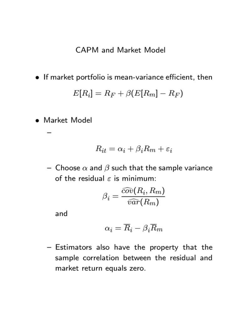
CAPM and Market Model
• If market portfolio is mean-variance efficient, then
E[Ri] = RF + β(E[Rm] − RF )
• Market Model
—
Rit = αi + β iRm + εi
— Choose α and β such that the sample variance
of the residual ε is minimum:
and
d
cov(R
i, Rm)
βi =
d
var(R
m)
αi = Ri − β iRm
— Estimators also have the property that the
sample correlation between the residual and
market return equals zero.
— Summary of properties
∗ Unsystematic risk is minimum
∗ Average residual is zero so the average stock
and market return fall on regression line
∗ Sample correlation between residual and market return equals zero
— Residual across stocks may be correlated, suggesting that additional factors may be required
• CAPM and Market Model
— Assume market model beta and CAPM beta
are the same.
— Then the CAPM places restriction on the value
of α.
— Under market model:
E[R] = α + βE[Rm]
— Therefore,
α = RF (1 − β)
— If β > 1, α < 0
— If β < 1, α > 0
• Example
— Suppose E[Rm] = 10% and RF = 6%.
— Consider four stocks with betas of 0, .5, 1,
and 1.5.
— If CAPM holds, then alphas are given by 6%,
3%, 0, −3%
-4
15
15
10
R
10
E[R]
5
5
-2 0
2
4
6
Rm
8
10
12
0
-5
-5
-10
-10
0.5
1
beta
1.5
2
• — In up market, high beta stocks tend to perform
better
— For example, suppose Rm = 20%
30
25
20
E[R|Rm=20]
15
10
5
0
0.5
1
beta
1.5
2
• — In down market, low beta stocks tend to perform better
— For example, Rm = −5%
10
5
0
0.5
beta
1
1.5
2
-5
E[R|Rm=-5]
-10
-15
• — But over up and down markets, high beta
stocks have higher average returns
• — Flat relationship: alphas given by 10%, 5%,
0%, -5%
15
10
R
5
-5
0
5
Rm
10
15
-5
-10
• — Given that for large portfolios,
σ 2p = β 2pσ 2m +
+
N µ ¶2
X
1
j=1 N
X X µ 1 ¶2
j6=k
N
cov(εj , εk )
var(εi)
2
2
= β pσ m +
+
N
var(εi)
µ
¶
1 2
(N 2 − N)cov(εj , εk )
N
var(εi)
1
= β 2pσ 2m +
+ cov(εj , εk )(1 − )
N
N
—
lim σ 2p = β 2pσ 2m + cov(εj , εk )
N →∞
— a portfolio of low beta stocks will have lower
total risk.
— For a flat relationship, risk averse investors will
choose low-beta risky portfolio and adjust risk
by borrowing or lending at risk-free rate.
— If expected return on a portfolio is greater than
risk-free rate, one can always increase the expected return and beta with leverage.
— Suppose β U is beta of unlevered portfolio,
then beta of levered portfolio is
β L = Xβ U + (1 − X)(0)
— Expected return is given by
E[RLEV ] = RF + X(E[Rm] − RF )
— So
βL
E[RLEV ] = RF +
(E[Rm] − RF )
βU
— If unlevered portfolio is the market,
E[RLEV ] = RF + β L(E[Rm] − RF )
— Also,
σ LEV
βL = X =
σm